The
Thermohaline Ocean Circulation
A Brief Fact Sheet
- by Stefan Rahmstorf
For an updated and more detailed version,
see the following paper (pdf, 3MB):
Rahmstorf,
S., 2006: Thermohaline Ocean Circulation. In: Encyclopedia of Quaternary
Sciences, Edited by S. A. Elias. Elsevier, Amsterdam.

What is the thermohaline circulation (THC)?
As opposed to wind-driven currents and tides (which are due to the gravity of moon and sun), the thermohaline circulation (Fig. 1) is that part of the ocean circulation which is driven by density differences. Sea water density depends on temperature and salinity, hence the name thermo-haline. The salinity and temperature differences arise from heating/cooling at the sea surface and from the surface freshwater fluxes (evaporation and sea ice formation enhance salinity; precipitation, runoff and ice-melt decrease salinity). Heat sources at the ocean bottom play a minor role.  |
Figure 1. Schematic
representation of the global thermohaline circulation.
Surface currents are shown
in red, deep waters in light blue and bottom waters in dark
blue. The main deep water formation sites are shown in orange.
(After [1], modified by S.R.)
|
In contrast to the wind-driven currents, the THC is not confined to surface waters but can be regarded as a big overturning of the world ocean, from top to bottom. The thermohaline circulation consists of:
- Deep water formation: the sinking of water masses, closely associated with (but not to be confused with) convection, which is a vertical mixing process, [2]). Deep water formation takes place in a few localised areas: the Greenland-Norwegian Sea, the Labrador Sea, the Mediteranean Sea, the Wedell Sea, the Ross Sea.
- Spreading of deep waters (e.g., North Atlantic Deep Water, NADW, and Antarctic Bottom Water, AABW), mainly as deep western boundary currents (DWBC).
- Upwelling of deep waters: this is not as localised and difficult to observe. It is thought to take place mainly in the Antarctic Circumpolar Current region, possibly aided by the wind (Ekman divergence).
- Near-surface currents: these are required to close the flow. In the Atlantic, the surface currents compensating the outflow of NADW range from the Benguela Current off South Africa via Gulf Stream and North Atlantic Current into the Nordic Seas off Scandinavia (Fig. 2). (Note that the Gulf Stream is primarily a wind-driven current, as part of the subtropical gyre circulation. The thermohaline circulation contributes only roughly 20% to the Gulf Stream flow.)
 |
| Figure 2. Thermohaline circulation of the
Atlantic. This highly simplified cartoon of Atlantic currents shows warmer surface currents (red) and cold north Atlantic Deep Water (NADW, blue). The thermohaline circulation heats the North Atlantic and Northern Europe. It extends right up to the Greenland and Norwegian Seas, pushing back the winter sea ice margin. (From [3].) |
Some observational data
The volume transport of the overturning circulation at 24 N has been estimated from hydrographic section data ([4]) as 17 Sv (1 Sv = 106 m3/s), its heat transport as 1.2 PW (1 PW = 1015 W). More recently, an inverse model by [5] yielded 15+-2 Sv NADW overturning in the high latitudes. (Note: when comparing these numbers with models care needs to be taken what exactly is compared - in models, the most common measure of NADW overturning is the maximum of the zonally integrated transport stream function in the North Atlantic, sometimes also the outflow value at 30 S.)
What drives the THC?
The short answer would be: high-latitude
cooling. In cold regions the highest surface water densities are
reached, this causes convective mixing and sinking of deep water,
which drives the circulation. Reality is more complex. Pressure gradients at depth, resulting from density gradients in the overlying waters, are the driving force in the equations of motion. As the density forcing occurs at the surface (see above), a subtle question is why the density differences and the circulation affect the whole ocean depth and are not confined to a near-surface layer. [6] showed that a deep circulation only arises when heating (buoyancy source) is at depth and cooling at the surface. The reason that there is a deep circulation after all is turbulent mixing, which brings down the heat on a time scale of ~1000 years. It has been shown that in the long-term equilibrium the strength of the thermohaline circulation in models depends on the turbulent mixing coefficient [7], and that the energy required for this turbulent mixing comes to a large extent from the moon via tidal currents ([8]).
This discussion can be labelled: is the THC pushed or pulled ([9])? I.e., pushed by formation of cold deep water, or pulled by downward diffusion of heat through the thermocline? The answer is a question of time scale: ultimately, in the long run, it is pulled. But on shorter time scales, up to centuries, it can be considered pushed in the sense that it is density changes in the deep water formation regions which affect the circulation strength. If this density drops too much so that deep water formation is not possible, the circulation stops. Ultimately, on the long time scale of turbulent mixing, the deep ocean density will drop as well until new deep water formation can start.
Non-linear behaviour of the
THC
As mentioned above, highest surface
densities in the world ocean are reached where water is very cold,
while lower densities are found in the saltier but warmer tropical
and subtropical areas. In this sense the THC is thermally driven.
Nevertheless, the influence of salinity is important and is what causes
the non-linearity of the system. This was first described in a classic
paper by [10] with the help of a simple box model. Salinity is involved
in a positive feedback: higher salinity in the deep water formation
area enhances the circulation, and the circulation in turn transports
higher salinity waters into the deep water formation regions (which
tend to be regions of net precipitation, i.e., freshwater would accumulate
and surface salinity would drop if the circulation stopped). Put simply,
in Stommel's model the high-latitude salinity increases linearly with
the flow, and the flow increases linearly with high-latitude salinity,
which combined gives a quadratic (i.e., non-linear) equation. This
leads to two possible equilibrium states, the system is bistable
in a certain parameter range. This becomes more than an academic point
as complex circulation models behave in the same way, and as the present
North Atlantic in many models is in the bistable regime ([11]). The
first coupled climate model to show these two equilibria (discovered
quite by accident) is the one by [12]. The situation can be described with a simple stability diagram showing strength of the THC as a function of the freshwater input into the North Atlantic. This shows the bistable regime and a saddle-node bifurcation point where the circulation breaks down. It is discussed in more detail (but for the non-specialist) in [13].
An important point is that the salt transport feedback is not the only feedback rendering the system non-linear. The convective mixing process is itself a highly non-linear, self-sustaining process. In models this can lead to multiple stable convection patterns ([14, 15]), which on one hand can cause artefacts related to the coarse model grid. On the other hand this may be part of a real mechanism for shifts in convection location, as have apparently occured during glacial times.
The bottom line is: salinity leads to non-linearity which causes the existence of multiple equilibria and thresholds in the THC.
A related question is: why is no deep water formed in the North Pacific? Salinity there is too low, but why? A body of literature exists on this topic; it is discussed e.g. in [16]. My opinion is: for geographical reasons so much freshwater enters the North Pacific that it is far in the monostable regime where no deep water formation is possible.
The effect on climate
The climatic effect of the THC
is still to some extent under discussion, and is due to the heat
transport of ~1 PW of this circulation. Back-of-the-envelope calculations
suggest that this amount of heat transported into the northern North
Atlantic (north of 24 N) should warm this region by ~5K. This is indeed
roughly the difference between sea surface temperature (SST) in the
North Atlantic as compared to the North Pacific at similar latitudes.
A look at sea ice margins suggest that they are pushed back by the
warm surface currents in the Atlantic sector as compared to the North
Pacific (Fig. 1), this in turn leads to reduced reflection of sunlight
and thus warming (albedo feedback). A look at global surface
air temperatures is also quite suggestive: over the three main deep
water formation regions of the world ocean, air temperatures are warmer
by up to ~10K compared to the latitudinal mean. These observations are, however, no quantitative proof of the climatic effect of the THC, and other explanations can be invoked, such as planetary waves in the atmosphere, locked in place by the geography (Rocky mountains).
One way to estimate the effect of the THC is to switch it off in coupled climate models (by adding a lot of freshwater to the northern Atlantic), and compare the surface climate before and after switching it off. Roughly, this leads to a cooling with a maximum of ~10K over the Nordic Seas (e.g., [12, 17]). The maximum tends to occur near the sea ice margin due to the ice albedo effect. Unfortunately, the details of this cooling are model-dependent: one model shows cooling up to 22K in annual mean and 33K in winter ([18]). Models also differ in how widespread the cooling is: most tend to affect temperatures over land in northwestern Europe (Scandinavia, Britain) by several degrees, others show strong cooling further west affecting Canada ([19]).
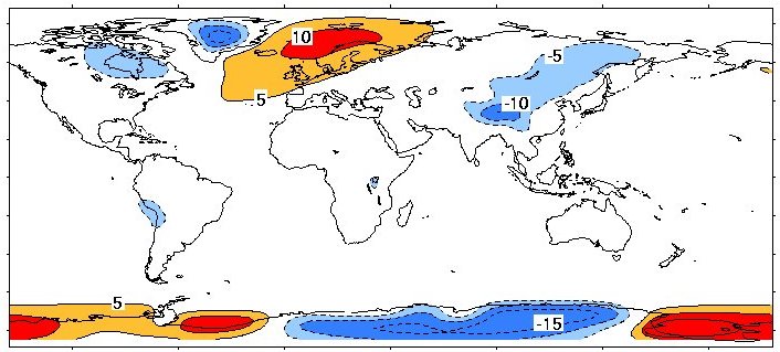 |
| Figure 3. Deviation of surface air temperature
from zonal mean. Deviations are shown in degree C. Based on NCAR surface air temperature climatology, reproduced from [20]. |
History of the THC
Sediment data document that the THC has undergone major
changes in the history of climate (e.g., [21, 22]). Three major circulation
modes were indentified: a warm mode similar to the present-day
Atlantic, a cold mode with NADW forming south of Iceland in the Irminger
Sea, and a switched-off mode ([23]). The latter appears to have occurred
after major input of freshwater, either from surging glacial ice sheets
(Heinrich events) or in form of meltwater floods (e.g., Younger
Dryas event). The most dramatic climate events recorded in Greenland,
the Dansgaard-Oeschger (D/O) events, were probably associated
with north-south shifts in convection location, i.e. transitions between
warm and cold modes of the Atlantic THC. Recent simulations of such
shifts show encouraging agreement with paleoclimatic data ([24]).
The THC in anthropogenic
global warming
Global warming can affect the
THC in two ways: surface warming and surface freshening,
both reducing the density of high-latitude surface waters and thus
inhibiting deep water formation. [25] was the first to warn that this
could lead to a breakdown of the THC and to abrupt climate change.
Subsequently, [26, 27] showed that this could indeed occur for strong
global warming (i.e., for a quadrupling, but not for a doubling of
CO2). In these scenarios there was no surface cooling,
as the high CO2 levels more than compensated for the reduced
ocean heat transport. The possibility of a real cooling (both a relative
cooling, i.e. a drop back to roughly pre-industrial temperatures after
an initial warming phase, and in the longer run an absolute
cooling below preindustrial values) as a result of anthropogenic warming
was first demonstrated in a sensitivity study by [20]. Significant
absolute cooling can arise after CO2 levels decline, but
the THC remains switched off after its collapse is triggered in a
rapid warming phase. A THC collapse is now widely discussed as one of a number of "low probability - high impact" risks associated with global warming. More likely than a breakdown of the THC, which only occurs in very pessimistic scenarios, is a weakening of the THC by 20-50%, as simulated by many coupled climate models ([28]).
Key open questions include:
- What changes in freshwater input to the North Atlantic will result from global warming? (Uncertainty e.g. due to uncertain estimates of Greenland meltwater runoff, ignored so far in most models, and due to possible changes in ENSO ([29]).)
- What is the risk of exceeding a threshold for THC collapse for a given warming?
- What other thresholds exist? (E.g., a local shutdown of convection in the Labrador Sea as simulated by [30], rather than a full THC collapse.)
- What consequences would result for marine ecosystems?
- How would temperatures over land be affected by a collapse scenario? (Just a reduced warming, or a warming followed by abrupt cooling?)
References
- Broecker, W.S., The great ocean conveyor. Oceanography, 1991. 4(2): p. 79-89.
- Send, U. and J. Marshall, Integral effects of deep convection. Journal of Physical Oceanography, 1995. 25: p. 855-872.
- Rahmstorf, S., Risk of sea-change in the Atlantic. Nature, 1997. 388: p. 825-826.
- Roemmich, D.H. and C. Wunsch, Two transatlantic sections: Meridional circulation and heat flux in the subtropical North Atlantic Ocean. Deep Sea Research, 1985. 32: p. 619-664.
- Ganachaud, A. and C. Wunsch, Improved estimates of global ocean circulation, heat transport and mixing from hydrographic data. Nature, 2000. 408: p. 453-457.
- Sandström, J.W., Dynamische Versuche mit Meerwasser. Annalen der Hydrographie und Maritimen Meteorologie, 1908. 36: p. 6-23.
- Bryan, F., Parameter sensitivity of primitive equation ocean general circulation models. Journal of Physical Oceanography, 1987. 17: p. 970-985.
- Wunsch, C., Moon, tides and climate. Nature, 2000. 405: p. 743-744.
- Robinson, A. and H. Stommel, The oceanic thermocline and the associated thermohaline circulation. Tellus, 1959. 11(3): p. 295-308.
- Stommel, H., Thermohaline convection with two stable regimes of flow. Tellus, 1961. 13: p. 224-230.
- Rahmstorf, S., On the freshwater forcing and transport of the Atlantic thermohaline circulation. Climate Dynamics, 1996. 12: p. 799-811.
- Manabe, S. and R.J. Stouffer, Two stable equilibria of a coupled ocean-atmosphere model. Journal of Climate, 1988. 1: p. 841-866.
- Rahmstorf, S., The thermohaline ocean circulation - a system with dangerous thresholds? Climatic Change, 2000. 46: p. 247-256.
- Rahmstorf, S., Bifurcations of the Atlantic thermohaline circulation in response to changes in the hydrological cycle. Nature, 1995. 378: p. 145-149.
- Rahmstorf, S., Rapid climate transitions in a coupled ocean-atmosphere model. Nature, 1994. 372: p. 82-85.
- Rahmstorf, S., J. Marotzke, and J. Willebrand, Stability of the thermohaline circulation, in The warm water sphere of the North Atlantic ocean, W. Krauss, Editor. 1996, Borntraeger: Stuttgart. p. 129-158.
- Manabe, S. and R.J. Stouffer, Are two modes of thermohaline circulation stable? Tellus, 1999. 51A: p. 400-411.
- Schiller, A., U. Mikolajewicz, and R. Voss, The stability of the thermohaline circulation in a coupled ocean-atmosphere general circulation model. Climate Dynamics, 1997. 13: p. 325-347.
- Vellinga, M. and R.A. Wood, Global climatic impacts of a collapse of the Atlantic thermohaline circulation. Climatic Change, 2002. 54: p. 251-267.
- Rahmstorf, S. and A. Ganopolski, Long-term global warming scenarios computed with an efficient coupled climate model. Climatic Change, 1999. 43: p. 353-367.
- Sarnthein, M., et al., Changes in east Atlantic deepwater circulation over the last 30,000 years: Eight time slice reconstructions. Paleoceanography, 1994. 9: p. 209-267.
- Sarnthein, M., et al., Variations in Atlantic surface paleoceanography, 50-80N: A time slice record of the last 30,000 years. Paleoceanography, 1995. 10: p. 1063-1094.
- Alley, R.B., et al., Making sense of millennial scale climate change, in Mechanisms of global climate change at millennial time scales, P.U. Clark, R.S. Webb, and L.D. Keigwin, Editors. 1999, AGU: Washington. p. 385-394.
- Ganopolski, A. and S. Rahmstorf, Rapid changes of glacial climate simulated in a coupled climate model. Nature, 2001. 409: p. 153-158.
- Broecker, W., Unpleasant surprises in the greenhouse? Nature, 1987. 328: p. 123.
- Manabe, S. and R.J. Stouffer, Century-scale effects of increased atmospheric CO2 on the ocean-atmosphere system. Nature, 1993. 364: p. 215-218.
- Manabe, S. and R.J. Stouffer, Multiple-century response of a coupled ocean-atmosphere model to an increase of atmospheric carbon dioxide. Journal of Climate, 1994. 7: p. 5-23.
- Rahmstorf, S., Shifting seas in the greenhouse? Nature, 1999. 399: p. 523-524.
- Latif, M., et al., Tropical stabilization of the thermohaline circulation in a greenhouse warming simulation. Journal of Climate, 2000. 13(11): p. 1809-1813.
- Wood, R.A., et al., Changing spatial structure of the thermohaline circulation in response to atmospheric CO2 forcing in a climate model. Nature, 1999. 399: p. 572-575.