
Technical Policy Briefing Notes - 4
Real Options Analysis
Description of the Method
Policy Briefs
Real Options Analysis
Description of the Method
The concepts of real options analysis lie originally in the
financial markets. A financial option gives the investor the right, but
not the obligation, to acquire a financial asset in the future,
allowing them to observe how market conditions play out before deciding
whether to exercise the option. This transfers risk from the buyer to
the seller, making the option a valuable commodity. Options analysis
quantifies this value based on how much such a risk transfer is worth
(Black and Scholes, 1973).
The same insights are also useful for investment in physical assets (hence ‘real’ options), in cases where there is risk/uncertainty (McDonald and Siegel, 1986). Real options analysis (ROA) quantifies the investment risk associated with uncertain future outcomes. It is particularly useful when considering the value of flexibility of investments. This might be for example flexibility over the timing of the original capital investment, or the flexibility to adjust the investment as it progresses over a number of stages, allowing decision-makers to adapt, expand or scale-back the project in response to unfolding events.
ROA typically gives two types of result that set it apart from traditional economic analysis. The first affects projects that are cost-efficient under a deterministic analysis. ROA shows that sometimes it makes more sense to wait for the outcome of new information, rather than investing immediately. Conversely, the second type of result affects projects which may fail a deterministic test of cost-efficiency. Under conditions of uncertainty, it may make financial sense to start the initial stages of the project where these are needed to keep the overall project alive, in case its fortunes change at a later date and it starts to look like an attractive investment option.
ROA has been applied quite widely in the energy sector, including analysis of mitigation options, and there are examples in the literature looking at the uncertainty of investment under climate change policy (e.g. Hlouskova et al. 2005: Fuss et al, 2009; Szolgayova et al 2011). As further examples, Rothwell (2006) examined returns on investment in nuclear plant with uncertainty over carbon prices, while Laurikka and Koljonen (2006) looked at investment uncertainty with future emissions trading.
Such studies show that ROA can provide useful information to help decisions in cases of three key conditions:
For a simple one-off investment opportunity which faces uncertain outcomes, it may be worth waiting to invest at a later date when more information is gained about the likelihood of different outcomes. Waiting can help the decision-maker to avoid costly mistakes by allowing them to decide not to proceed with an investment if they find themselves facing poor investment conditions.
For waiting to be worthwhile, the decision-maker must reasonably expect to gain valuable information. The value of waiting will then be higher (lower) if:
ROA therefore provides decision-makers with a new investment criterion that takes account of uncertainty. Projects should proceed if the project overall seems cost-efficient and if the cumulative lost value of these benefits during the waiting time exceeds the value of waiting.
However, projects are usually more complex than a simple one-off investment, and ROA can add to the understanding of how project value evolves during the various stages of project development.
There will often be flexibility to adapt the project as it proceeds through these stages, for example to expand, contract, or even stop the project altogether if it appears unlikely to be successful.
Standard economic appraisal normally assesses the performance of the project over its whole lifecycle without taking account of the value of this flexibility. Averaging the outcomes across multiple scenarios will tend to undervalue projects, because it does not take account of the ways in which projects can be adapted to adjust as these various scenarios arise over time. The advantage of ROA is that it can incorporate the value of this flexibility, and can therefore lead to better decision making (HMT, 2007).
ROA can be carried out in a variety of ways. The most relevant to adaptation is an approach called dynamic programming which is essentially an extension of decision-tree analysis. This defines possible outcomes, and assigns probabilities to these.
The decision-tree defines how a decision-maker responds to resolution of uncertainty at each branching point in the tree. Quantifying the value of these decision options then proceeds by assessing all the branches. ROA calculates option value based on the expected value over all branches contingent on making the optimal choice being taken at each decision-point.
The optimal decision in turn is evaluated based on all the possible outcomes downstream of that decision in the tree. This ROA value can be compared to a normal economic (cost-benefit) calculation that would simply be a probabilityweighted average of the outcomes along each possible branch in the tree.
The same insights are also useful for investment in physical assets (hence ‘real’ options), in cases where there is risk/uncertainty (McDonald and Siegel, 1986). Real options analysis (ROA) quantifies the investment risk associated with uncertain future outcomes. It is particularly useful when considering the value of flexibility of investments. This might be for example flexibility over the timing of the original capital investment, or the flexibility to adjust the investment as it progresses over a number of stages, allowing decision-makers to adapt, expand or scale-back the project in response to unfolding events.
ROA typically gives two types of result that set it apart from traditional economic analysis. The first affects projects that are cost-efficient under a deterministic analysis. ROA shows that sometimes it makes more sense to wait for the outcome of new information, rather than investing immediately. Conversely, the second type of result affects projects which may fail a deterministic test of cost-efficiency. Under conditions of uncertainty, it may make financial sense to start the initial stages of the project where these are needed to keep the overall project alive, in case its fortunes change at a later date and it starts to look like an attractive investment option.
ROA has been applied quite widely in the energy sector, including analysis of mitigation options, and there are examples in the literature looking at the uncertainty of investment under climate change policy (e.g. Hlouskova et al. 2005: Fuss et al, 2009; Szolgayova et al 2011). As further examples, Rothwell (2006) examined returns on investment in nuclear plant with uncertainty over carbon prices, while Laurikka and Koljonen (2006) looked at investment uncertainty with future emissions trading.
Such studies show that ROA can provide useful information to help decisions in cases of three key conditions:
- First, the investment decision is irreversible once taken;
- Second, the decision-maker has some flexibility when to carry out the investment (either in a single step, or in stages);
- Third, the decision-maker faces uncertain conditions and by waiting to invest they are able to gain new valuable information regarding the success of the investment.
For a simple one-off investment opportunity which faces uncertain outcomes, it may be worth waiting to invest at a later date when more information is gained about the likelihood of different outcomes. Waiting can help the decision-maker to avoid costly mistakes by allowing them to decide not to proceed with an investment if they find themselves facing poor investment conditions.
For waiting to be worthwhile, the decision-maker must reasonably expect to gain valuable information. The value of waiting will then be higher (lower) if:
- The degree of uncertainty regarding the costeffectiveness of the project is greater (smaller)
- The duration of the period of waiting before information is gained is shorter (longer)
ROA therefore provides decision-makers with a new investment criterion that takes account of uncertainty. Projects should proceed if the project overall seems cost-efficient and if the cumulative lost value of these benefits during the waiting time exceeds the value of waiting.
However, projects are usually more complex than a simple one-off investment, and ROA can add to the understanding of how project value evolves during the various stages of project development.
There will often be flexibility to adapt the project as it proceeds through these stages, for example to expand, contract, or even stop the project altogether if it appears unlikely to be successful.
Standard economic appraisal normally assesses the performance of the project over its whole lifecycle without taking account of the value of this flexibility. Averaging the outcomes across multiple scenarios will tend to undervalue projects, because it does not take account of the ways in which projects can be adapted to adjust as these various scenarios arise over time. The advantage of ROA is that it can incorporate the value of this flexibility, and can therefore lead to better decision making (HMT, 2007).
ROA can be carried out in a variety of ways. The most relevant to adaptation is an approach called dynamic programming which is essentially an extension of decision-tree analysis. This defines possible outcomes, and assigns probabilities to these.
The decision-tree defines how a decision-maker responds to resolution of uncertainty at each branching point in the tree. Quantifying the value of these decision options then proceeds by assessing all the branches. ROA calculates option value based on the expected value over all branches contingent on making the optimal choice being taken at each decision-point.
The optimal decision in turn is evaluated based on all the possible outcomes downstream of that decision in the tree. This ROA value can be compared to a normal economic (cost-benefit) calculation that would simply be a probabilityweighted average of the outcomes along each possible branch in the tree.
Box 1: The
Concepts of Real Options Analysis
The example below shows a simplified investment example, showing the expected gross margin over time, with annuitized capital costs shown as a blue shaded area. Uncertainty is represented as an anticipated shock or an information event that occurs in the future (Tp) which will affect the project’s cash flow either adversely (the red line) or favourably (the green line). In case A (top) – the normal positive NPV criterion – a decision has to be made at time t=0 on whether or not to invest. In this case, there is not the option to wait. The expected ‘best guess’ (the central orange line) is the average of the upper and lower estimate of the outcome of the price shock, noting in this case, risks are symmetrical, and cancel out such that the expected value of project will continue to be profitable (and thus the decision maker should proceed with the investment). In Case B (bottom), there is the opportunity to wait until time Tp before making the investment. This allows it to avoid the potential loss that might occur if conditions turn out worse than expected (the red dashed area), but this must be traded off against the opportunity costs of waiting (the orange dashed area).
The associated decision tree for this example is shown below. The ‘risk event’ represents an event in which a variable which was previously uncertain is resolved. In this example, there are only two equivalent outcomes, a high revenue scenario and a low revenue scenario, noting in practice, there may be many outcomes, with different probabilities.
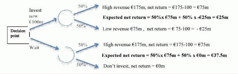 To make a direct
comparison between the ‘invest now’ and the
‘wait’ options, the expected net returns (the
probability weighted mean) is expressed in present value terms, since
the decisionmaker needs to compare the relative value of the two
options in the current time period of the decision. Under the
‘invest now’ branch, the expected net return in
present value terms is €25m, since revenue starts to flow
immediately. Under the ‘wait’ branch, the expected
net returns of €37.5m needs to be discounted. If the duration
of the wait was 3 years, and a discount rate of 7% is used, then the
present value would be €30.6m. In this case, the
decision-maker would better off waiting. If the duration of the wait
was 8 years, at 7% discount rate, the present value of the investment
option would be €22m, so the decision-maker in this case would
be better off to invest immediately, and take the future downside risk
when it occurs.
To make a direct
comparison between the ‘invest now’ and the
‘wait’ options, the expected net returns (the
probability weighted mean) is expressed in present value terms, since
the decisionmaker needs to compare the relative value of the two
options in the current time period of the decision. Under the
‘invest now’ branch, the expected net return in
present value terms is €25m, since revenue starts to flow
immediately. Under the ‘wait’ branch, the expected
net returns of €37.5m needs to be discounted. If the duration
of the wait was 3 years, and a discount rate of 7% is used, then the
present value would be €30.6m. In this case, the
decision-maker would better off waiting. If the duration of the wait
was 8 years, at 7% discount rate, the present value of the investment
option would be €22m, so the decision-maker in this case would
be better off to invest immediately, and take the future downside risk
when it occurs.
The example below shows a simplified investment example, showing the expected gross margin over time, with annuitized capital costs shown as a blue shaded area. Uncertainty is represented as an anticipated shock or an information event that occurs in the future (Tp) which will affect the project’s cash flow either adversely (the red line) or favourably (the green line). In case A (top) – the normal positive NPV criterion – a decision has to be made at time t=0 on whether or not to invest. In this case, there is not the option to wait. The expected ‘best guess’ (the central orange line) is the average of the upper and lower estimate of the outcome of the price shock, noting in this case, risks are symmetrical, and cancel out such that the expected value of project will continue to be profitable (and thus the decision maker should proceed with the investment). In Case B (bottom), there is the opportunity to wait until time Tp before making the investment. This allows it to avoid the potential loss that might occur if conditions turn out worse than expected (the red dashed area), but this must be traded off against the opportunity costs of waiting (the orange dashed area).
| Case A: “Now or never” investment option at t=0 |
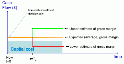 |
| Case B: Option to wait until after t=Tp, the expected time of policy change that affects the investment |
 |
The associated decision tree for this example is shown below. The ‘risk event’ represents an event in which a variable which was previously uncertain is resolved. In this example, there are only two equivalent outcomes, a high revenue scenario and a low revenue scenario, noting in practice, there may be many outcomes, with different probabilities.
 download this briefing note