In the extensive simulations we have conducted, the parameters for the present state of the
Earth system
(e.g. ![]() ) are used as starting values. By combining Eqs. 2
to 6
with Eq. 1, a relation is found which depends only on the surface temperature
) are used as starting values. By combining Eqs. 2
to 6
with Eq. 1, a relation is found which depends only on the surface temperature
![]() , and the atmospheric CO
, and the atmospheric CO![]() content
content ![]() .
The next step is to use the greenhouse model of Caldeira and Kasting[1] in order to
express
.
The next step is to use the greenhouse model of Caldeira and Kasting[1] in order to
express ![]() in
terms of
in
terms of ![]() . The resulting equation contains only
. The resulting equation contains only ![]() as an unknown variable.
The root of this equation yields the equilibrium solution of the atmospheric CO
as an unknown variable.
The root of this equation yields the equilibrium solution of the atmospheric CO![]() content,
content,
![]() . Finally, the equilibrium values of
. Finally, the equilibrium values of ![]() ,
, ![]() , and
, and
![]() can be calculated.
This is the solution for the present state of our Earth system.
can be calculated.
This is the solution for the present state of our Earth system.
To perform the calculations at any other
time, one has to use the time-dependent solar insolation (Eq. 3) and a possible change
of the
dimensionless weathering rate. The value of ![]() can be determined from the
ratio of the dimensionless
mid-ocean sea-floor spreading rate and the dimensionless continental area from Franck
and Bounama[30, 31] via Eq. 10. Applying the procedure
described above, we run our model back to the Proterozoic. At this geological era, life had
already changed
from anaerobic to aerobic forms, so from that time on the biological productivity can be
described by
Eq. 6. Starting from the present state again, we run our model 1.5 Ga into the
future. This is done
by extrapolating the present day continental-growth rate and by calculating the spreading rate
according to
Franck and Bounama[31]. In addition, we performed the whole procedure also for different
orbital distances
between Earth and Sun.
can be determined from the
ratio of the dimensionless
mid-ocean sea-floor spreading rate and the dimensionless continental area from Franck
and Bounama[30, 31] via Eq. 10. Applying the procedure
described above, we run our model back to the Proterozoic. At this geological era, life had
already changed
from anaerobic to aerobic forms, so from that time on the biological productivity can be
described by
Eq. 6. Starting from the present state again, we run our model 1.5 Ga into the
future. This is done
by extrapolating the present day continental-growth rate and by calculating the spreading rate
according to
Franck and Bounama[31]. In addition, we performed the whole procedure also for different
orbital distances
between Earth and Sun.
The results for the mean global surface temperature ![]() and the normalized biological
productivity
and the normalized biological
productivity
![]() are plotted in Figs. 2 and 3, respectively. Fig. 2 compares the evolution of the
mean global surface
temperature from the Proterozoic up to the planetary future for the geostatic model (GSM)
and for
our geodynamical model (GDM). Up to 1 Ga into the future, the temperature varies only
within
an interval of
are plotted in Figs. 2 and 3, respectively. Fig. 2 compares the evolution of the
mean global surface
temperature from the Proterozoic up to the planetary future for the geostatic model (GSM)
and for
our geodynamical model (GDM). Up to 1 Ga into the future, the temperature varies only
within
an interval of ![]() to
to ![]() . This stabilization of the surface temperature is
a
result of the
carbonate-silicate self-regulation within the Earth system with respect to growing insolation as
an external forcing.
. This stabilization of the surface temperature is
a
result of the
carbonate-silicate self-regulation within the Earth system with respect to growing insolation as
an external forcing.

Figure 2: Past and future variation of the mean global surface temperature ![]() for
the four employed models:
GSM-asymptotic (+), GDM-asymptotic (
for
the four employed models:
GSM-asymptotic (+), GDM-asymptotic (![]() ), GSM-parabolic (
), GSM-parabolic (![]() ), and
GDM-parabolic (
), and
GDM-parabolic (![]() ).
The two parabolic models have multiple solutions in the past. The horizontal dashed
line indicates the ``optimal'' biogeophysical temperature, i.e.,
).
The two parabolic models have multiple solutions in the past. The horizontal dashed
line indicates the ``optimal'' biogeophysical temperature, i.e., ![]() .
.
In contrast to the GSM approach, the GDM scheme shows a temperature stabilization at a
higher
level in the past and a lower one in the future (see Fig. 2). This result is found
for the asymptotic biospheric productivity (Eq. 7) as well as for the parabolic one
described by Eq. 8.
Values before 2 Ga ago are not shown because at these times the GDM gives
atmospheric CO![]() concentrations higher than
concentrations higher than ![]() ppm. Under the latter conditions the
greenhouse model employed
is not valid. Nevertheless, both models show a good stabilization of the mean global
surface temperature
ppm. Under the latter conditions the
greenhouse model employed
is not valid. Nevertheless, both models show a good stabilization of the mean global
surface temperature ![]() against increasing insolation. In the far future near 1 Ga from
now, all curves converge
and show a strong increase in
against increasing insolation. In the far future near 1 Ga from
now, all curves converge
and show a strong increase in ![]() to almost
to almost ![]() . All higher forms of life,
especially the
photosynthesis-based biosphere, will certainly be extinguished at this time. This kind of
sensitivity was also discussed for other continental-growth models in previous papers
[31, 23].
. All higher forms of life,
especially the
photosynthesis-based biosphere, will certainly be extinguished at this time. This kind of
sensitivity was also discussed for other continental-growth models in previous papers
[31, 23].
During the long-term evolution of the Earth system, the development of the normalized biological productivity (Fig. 3) shows a remarkably different behaviour for the asymptotic and the parabolic models, respectively.
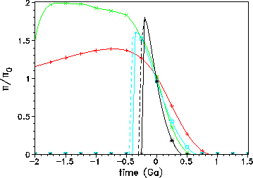
Figure 3:
Past and future variation of the normalized biological productivity ![]() for our four Earth system models.
Note that the two parabolic models have multiple solutions in the past (see also Fig. 2). The
dashed branch lines correspond
to backward-directed evolutions.
for our four Earth system models.
Note that the two parabolic models have multiple solutions in the past (see also Fig. 2). The
dashed branch lines correspond
to backward-directed evolutions.
Because of the chosen set of parameters used in Eq. 8,
both parabolic models (GSM and GDM) have zero productivities for times earlier than
500 Ma before present. This obviously contradicts the geological record. Therefore, in the
following, we will restrict ourselves to asymptotic models only.
In the past, these models generate higher values of ![]() than today. Our favoured
model, the
GDM-asymptotic model, calculates twice the present biological productivity for most of the
Proterozoic.
This seems reasonable because of the higher mean global surface temperatures at that time.
As continental growth starts late in our GDM-asymptotic model, the latter generates a strong
increase
in the biological productivity in the Proterozoic. This model also provides the shortest life
span of
the photosynthesis-based biosphere - nearly 300 Ma shorter than the corresponding
GSM-asymptotic model!
than today. Our favoured
model, the
GDM-asymptotic model, calculates twice the present biological productivity for most of the
Proterozoic.
This seems reasonable because of the higher mean global surface temperatures at that time.
As continental growth starts late in our GDM-asymptotic model, the latter generates a strong
increase
in the biological productivity in the Proterozoic. This model also provides the shortest life
span of
the photosynthesis-based biosphere - nearly 300 Ma shorter than the corresponding
GSM-asymptotic model!
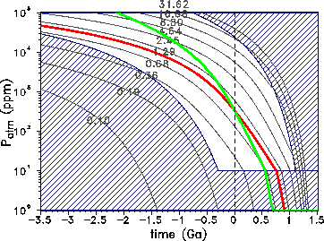
Figure 4: Evolution of the atmospheric carbon content as described by the models
GSM-asymptotic
(red line) and GDM-asymptotic (green line). The terrestrial life corridor (Eq. 14) is
identical to the
non-dashed region. The plotted isolines are the solutions of GSM-asymptotic for the
indicated fixed values of the normalized weathering rate ![]() .
.
Fig. 4 shows the atmospheric carbon content over geologic time from the Hadean to the
planetary
future for the two asymptotic models. In the dashed region of Fig. 4 no photosynthesis is
possible
because of inappropriate temperature or atmospheric carbon content. The non-dashed region
is
the ``terrestrial life corridor (TLC)''. Formally, the life corridor in the (![]() ,
,
![]() )-domain
is defined as
)-domain
is defined as
![]()
For the asymptotic model we have (inserting Eqs. 6, 7, and 9 into
Eq. 13):
![]()
It is possible to map TLC in different parameter spaces. For instance, ![]() can be substituted
with the help of the greenhouse
model by
can be substituted
with the help of the greenhouse
model by ![]() . Therefore, TLC can be depicted in the
(
. Therefore, TLC can be depicted in the
(![]() , t)-domain,
as shown in Fig. 4. The reference model GSM is based on a weathering rate that is
always equal to the present-day rate
, t)-domain,
as shown in Fig. 4. The reference model GSM is based on a weathering rate that is
always equal to the present-day rate ![]() .
The GDM takes into account the influence of a growing continental area and the changing
spreading rate on weathering. The GDM has higher weathering rates for the past
(i.e.
.
The GDM takes into account the influence of a growing continental area and the changing
spreading rate on weathering. The GDM has higher weathering rates for the past
(i.e. ![]() ). This can be explained easily with the help
of Eq. 10,
because in the geological past we had higher spreading rates
). This can be explained easily with the help
of Eq. 10,
because in the geological past we had higher spreading rates ![]() and a smaller
continental
area
and a smaller
continental
area ![]() . In the planetary future we find the
reversed situation: lower spreading rates and higher continental area will reduce the
atmospheric carbon content,
and this is the reason why the biosphere`s life span is significantly shorter because
photosynthesis can persist
only down to the critical level of 10 ppm atmospheric CO
. In the planetary future we find the
reversed situation: lower spreading rates and higher continental area will reduce the
atmospheric carbon content,
and this is the reason why the biosphere`s life span is significantly shorter because
photosynthesis can persist
only down to the critical level of 10 ppm atmospheric CO![]() concentration. As mentioned
above,
the GDM model does not work at atmospheric CO
concentration. As mentioned
above,
the GDM model does not work at atmospheric CO![]() concentrations higher than
concentrations higher than ![]() ppm, and
therefore the model fails on time scales of about 2 Ga ago. Compared to the
smooth curve of the GSM-asymptotic model, our favoured model (GDM-asymptotic)
provides a
curve with a certain structure that is directly related to the step-like continental growth shown
in
Fig. 1.
ppm, and
therefore the model fails on time scales of about 2 Ga ago. Compared to the
smooth curve of the GSM-asymptotic model, our favoured model (GDM-asymptotic)
provides a
curve with a certain structure that is directly related to the step-like continental growth shown
in
Fig. 1.
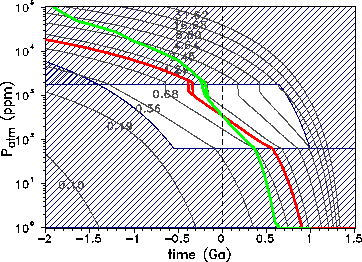
Figure 5: Evolution of the atmospheric carbon content as described by the models
GSM-parabolic
(red line) and GDM-parabolic (green line). The terrestrial life corridor for the parabolic model
is defined by
![]() and is identical
to the
non-dashed region. The plotted isolines have the same meaning as in Fig. 4.
and is identical
to the
non-dashed region. The plotted isolines have the same meaning as in Fig. 4.
The life corridor for the two parabolic models is plotted in Fig. 5. As already mentioned
above,
these models do not work very well for the past because the upper boundary for the
atmospheric
CO![]() content is rather low, between
content is rather low, between ![]() and
and ![]() ppm. Nevertheless, both curves
show the phenomenon
of bistability in the Phanerozoic. Dependent on the time direction, there are different
evolutionary paths in
the diagram. Such a hysteresis, in a much more pronounced form, can also be
calculated for the Daisyworld model class [20]. Similar effects were
discussed by Kump and Volk[18]. They found both bistability and insufficient
conditions for life for times of more than
100 Ma ago for the parabolic model, which is clearly not realistic.
ppm. Nevertheless, both curves
show the phenomenon
of bistability in the Phanerozoic. Dependent on the time direction, there are different
evolutionary paths in
the diagram. Such a hysteresis, in a much more pronounced form, can also be
calculated for the Daisyworld model class [20]. Similar effects were
discussed by Kump and Volk[18]. They found both bistability and insufficient
conditions for life for times of more than
100 Ma ago for the parabolic model, which is clearly not realistic.
Besides calculating the TLC, i.e., the evolution of atmospheric carbon regimes supporting photosynthetis-based life in time, we calculated the behaviour of our virtual Earth system at various distances from the Sun, using different insolations. Hart[34, 35] calculated the evolution of the terrestrial atmosphere over geologic time by varying the distance from the Sun. In his approach, the habitable zone (HZ) is the region within which an Earth-like planet might enjoy moderate surface temperatures needed for advanced life forms. Kasting et al.[40] defined the HZ of an Earth-like planet as the region where liquid water is present at the surface. According to this definition the inner boundary of the HZ is determined by the loss of water via photolysis and hydrogen escape. Kasting et al.[40] propose three definitions of the outer boundary of the HZ. All of them are connected to a surface-temperature limit of 273 K. This is in agreement with our definition of the low-temperature boundary of the biological productivity.
According to Kasting et al.[40] the outer boundary of the HZ is determined by CO![]() clouds
that attenuate the incident sunlight by Rayleigh scattering. The critical CO
clouds
that attenuate the incident sunlight by Rayleigh scattering. The critical CO![]() partial pressure
for the onset of this effect is about 5 to 6 bar (Kasting, personal communication, 1999). On the other hand,
the effects of CO
partial pressure
for the onset of this effect is about 5 to 6 bar (Kasting, personal communication, 1999). On the other hand,
the effects of CO![]() clouds have been challenged recently by Forget and Pierrehumbert[28]. CO
clouds have been challenged recently by Forget and Pierrehumbert[28]. CO![]() clouds
have the additional effect of reflecting the outgoing thermal radiation back to the surface. In this
way, they could have extended the size of the HZ in the past.
clouds
have the additional effect of reflecting the outgoing thermal radiation back to the surface. In this
way, they could have extended the size of the HZ in the past.
Hart[34, 35] found
that the HZ between runaway greenhouse and runaway
glaciation is surprisingly narrow for G2 stars like our Sun: ![]() AU,
AU,
![]() AU (AU = astronomical unit). A main disadvantage of these
calculations is the
neglect of the negative feedback between atmospheric CO
AU (AU = astronomical unit). A main disadvantage of these
calculations is the
neglect of the negative feedback between atmospheric CO![]() content and mean global
surface temperature discovered
later by Walker et al.[7]. The implementation of this feedback by Kasting et al.[39]
provides an almost constant inner boundary (
content and mean global
surface temperature discovered
later by Walker et al.[7]. The implementation of this feedback by Kasting et al.[39]
provides an almost constant inner boundary (![]() AU)
but a remarkable
extension of the outer boundary beyond Martian distance (
AU)
but a remarkable
extension of the outer boundary beyond Martian distance (![]() AU). Later Kasting et al.[40]
and Kasting et al.[38] recalculated the HZ boundaries as
AU). Later Kasting et al.[40]
and Kasting et al.[38] recalculated the HZ boundaries as ![]() AU and
AU and ![]() AU.
AU.
In a recent paper, Williams and Kasting[53] investigated the problem of habitable planets
with high obliquities with the help of an energy-balance climate model. In their
two-dimensional
model ![]() shifts to
shifts to ![]() AU. In our approach, the HZ for an
Earth-like planet is the
region within which the biological productivity is greater than zero. This is the region where
the surface temperature stays between
AU. In our approach, the HZ for an
Earth-like planet is the
region within which the biological productivity is greater than zero. This is the region where
the surface temperature stays between ![]() and
and ![]() and the atmospheric
CO
and the atmospheric
CO![]() content is higher than 10 ppm suitable for photosynthetis-based life. The term
``Earth-like''
explicitly implies also the occurrence of plate tectonics.
In order to assess the HZ, the life corridor is calculated by varying the distance of our
Earth-like
planet to the Sun for various time steps in the past, the present, and the future. Fig. 6 shows
the
results for the present state of the Earth system.
content is higher than 10 ppm suitable for photosynthetis-based life. The term
``Earth-like''
explicitly implies also the occurrence of plate tectonics.
In order to assess the HZ, the life corridor is calculated by varying the distance of our
Earth-like
planet to the Sun for various time steps in the past, the present, and the future. Fig. 6 shows
the
results for the present state of the Earth system.
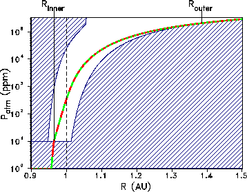
Figure 6: Present habitable zone (non-dashed region) for GSM-asymptotic (red)
and GDM-asymptotic (green). The two models provide identical answers as they are both
fitted to the same present-day parameters. Present inner and outer boundaries are determined
as ![]() AU and
AU and ![]() AU, respectively.
AU, respectively.
In this case, GSM and GDM give identical
curves because both models are fitted to the same present parameters. We find
![]() AU, so
our Earth system is even closer to a runaway greenhouse effect than in the calculations of
Hart[35]
and Kasting et al.[39]. The outer boundary is extended in comparison to the model
of
Hart[35], but not beyond the Martian distance (
AU, so
our Earth system is even closer to a runaway greenhouse effect than in the calculations of
Hart[35]
and Kasting et al.[39]. The outer boundary is extended in comparison to the model
of
Hart[35], but not beyond the Martian distance (![]() AU).
Despite the different
ansatz, our results are comparable to those found by Kasting et al.[40],
Kasting et al.[38], and Williams and Kasting[53].
AU).
Despite the different
ansatz, our results are comparable to those found by Kasting et al.[40],
Kasting et al.[38], and Williams and Kasting[53].
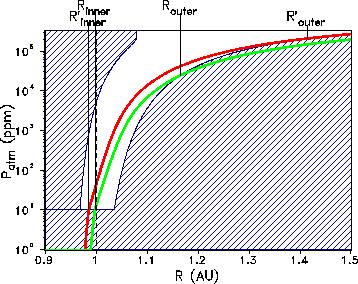
Figure 7: The habitable zone (non-dashed region) for an Earth-like planet in the ``near''
future
(0.5 Ga). For GDM-asymptotic (green line) the respective boundaries are
![]() AU and
AU and ![]() AU. Because
AU. Because
![]() will exactly coincide with the actual
distance of planet Earth from the Sun (1 AU), the life span of the biosphere will end at this
time. For GSM-asymptotic (red line) the respective boundaries are
will exactly coincide with the actual
distance of planet Earth from the Sun (1 AU), the life span of the biosphere will end at this
time. For GSM-asymptotic (red line) the respective boundaries are
![]() AU and
AU and ![]() AU.
AU.
In the planetary future at 0.5 Ga from now, the situation has changed dramatically (see Fig. 7: the geodynamic Earth-system
model GDM predicts that the lower boundary for atmospheric CO![]() concentration has
been reached already (
concentration has
been reached already (![]() AU),
and the boundary for a runaway glaciation has moved significantly inward
(
AU),
and the boundary for a runaway glaciation has moved significantly inward
(![]() AU).
Our results for the estimation of the HZ for all times are summarized in Fig. 8, where we have
plotted the width
and position of the HZ for the GSM and GDM variants over time.
AU).
Our results for the estimation of the HZ for all times are summarized in Fig. 8, where we have
plotted the width
and position of the HZ for the GSM and GDM variants over time.
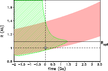
Figure 8: Evolution of the habitable zone (HZ) for GSM-asymptotic (red line) and
GDM-asymptotic (green line). Note that for GSM-asymptotic the HZ has a slightly increasing
width and shifts outward from the Sun. The HZ for our favoured model,
GDM-asymptotic, is both shifting and narrowing over geologic time, terminating life definitely
at 1.4 Ga. The
optimum position for an Earth-like planet would be at ![]() AU. In
this case the life span of the biosphere would realize the maximum life span, i.e. the
above-mentioned 1.4 Ga.
This figure is the main finding of our investigation.
AU. In
this case the life span of the biosphere would realize the maximum life span, i.e. the
above-mentioned 1.4 Ga.
This figure is the main finding of our investigation.
For the geostatic case (GSM) the width of the HZ slightly increases and shifts outward over
time. In about 800 Ma the inner boundary ![]() reaches the Earth
distance from the Sun (R = 1 AU) and the
biosphere ceases to exist, as already found above for this model. Our geodynamic model
shows both a shift and a narrowing of the HZ: the inner boundary
reaches the Earth
distance from the Sun (R = 1 AU) and the
biosphere ceases to exist, as already found above for this model. Our geodynamic model
shows both a shift and a narrowing of the HZ: the inner boundary ![]() reaches the Earth distance
in about 500 Ma from now in correspondence with the shortening of the life span of the
biosphere by about
300 Ma as compared to the geostatic model. In the GDM, the outer boundary
reaches the Earth distance
in about 500 Ma from now in correspondence with the shortening of the life span of the
biosphere by about
300 Ma as compared to the geostatic model. In the GDM, the outer boundary
![]() decreases in a strong nonlinear
way. This result is in contrast to the GSM and to the results of Kasting et al.[40] and
Kasting[38]. Since our criteria for the HZ is defined using biological productivity alone, the critical boundaries can be
extended for the temperature
from
decreases in a strong nonlinear
way. This result is in contrast to the GSM and to the results of Kasting et al.[40] and
Kasting[38]. Since our criteria for the HZ is defined using biological productivity alone, the critical boundaries can be
extended for the temperature
from ![]() to
to ![]() or higher. But our results show that the inner boundary
of the HZ is
determined by the 10 ppm limit (Fig. 6 and 7) and the outer boundary by the
or higher. But our results show that the inner boundary
of the HZ is
determined by the 10 ppm limit (Fig. 6 and 7) and the outer boundary by the ![]() limit.
limit.
Of course, there may exist chemolithoautotrophic hyperthermophiles that might survive even in a
future of higher temperatures, rather independently of atmospheric CO![]() pressures. But all higher
forms of life would certainly be eliminated under such conditions. Our biosphere model is actually only
relevant to photosynthesis-based life.
Therefore, in the time span under consideration, the upper temperature does not affect the
results for TLC and HZ, respectively.
pressures. But all higher
forms of life would certainly be eliminated under such conditions. Our biosphere model is actually only
relevant to photosynthesis-based life.
Therefore, in the time span under consideration, the upper temperature does not affect the
results for TLC and HZ, respectively.
The main objective of our paper is to generate model results for
the dependence of the biosphere life span on the sea-floor spreading rate
and the history of continent growth. Therefore, sensitivity tests based on the
variations of these geodynamics entities
have been performed. In Fig. 9, the ensemble of alternative
continental-growth models is sketched. The linear
and the delayed growth models reflect the simplest theoretical
assumptions [31]. The model of Reymer and Schubert[46] is based
on the assumption of an approximately constant continental
freeboard. For all of these models surface temperature, CO![]() history,
and biological productivity have been already investigated by
Franck et al.[23] in a recent study. Furthermore, we added a model with
constant continental area which seems to be in
contrast to geological records. Therefore, this geodynamic scenario is the most
unrealistic one. In all cases, the spreading rates are
calculated with the help of Eq. 11.
history,
and biological productivity have been already investigated by
Franck et al.[23] in a recent study. Furthermore, we added a model with
constant continental area which seems to be in
contrast to geological records. Therefore, this geodynamic scenario is the most
unrealistic one. In all cases, the spreading rates are
calculated with the help of Eq. 11.
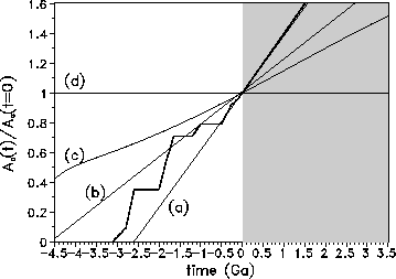
Figure 9: Normalized continental area ![]() as a consequence of the following continental-growth models: (a) delayed growth, (b) linear growth, (c) Reymer and Schubert, (d) constant area. The thick line indicates the Condie model (see Fig. 1).
as a consequence of the following continental-growth models: (a) delayed growth, (b) linear growth, (c) Reymer and Schubert, (d) constant area. The thick line indicates the Condie model (see Fig. 1).
Fig. 10 summarizes the results for the HZs for the additional four continental-growth scenarios indicated in Fig. 9. It is obvious that in all cases the life span of the biosphere is significantly shorter than in the GSM and the magnitude remains approximately the same for all alternatives (Table 1). The optimum distances for an Earth-like planet vary slightly between 1.09 and 1.21 AU. The maximum life span at the optimum distance varies between 1.35 and 2.05 Ga in cases a, b, and c, respectively, evidently increasing with decreasing continental-growth rate. In the most unrealistic case without continental growth but geodynamics, i.e. scenario d, the maximum life span is extended to 2.98 Ga.
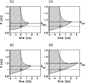
Figure 10: Habitable zones of the GDM-asymptotic for the four alternative continental-growth models: (a) delayed growth, (b) linear growth, (c) Reymer and Schubert, (d) constant area. Obviously, the so-calculated HZs do not differ in their qualitative
behaviour. The biosphere life span varies only slightly in magnitude and is
always shorter than in the geostatic case (GSM). Exact values for the biosphere life span, the optimum distance, and the maximum life span, respectively, can be found in
Table 1.
| Continental growth model | Biosphere life span (Ga) | | Maximum life span (Ga) |
| Delayed growth | 0.48 | 1.09 | 1.35 |
| Condie | 0.48 | 1.08 | 1.40 |
| Linear growth | 0.53 | 1.11 | 1.80 |
| Reymer and Schubert | 0.58 | 1.13 | 2.05 |
| Constant area | 0.63 | 1.19 | 2.98 |
The comparison of Figs. 8 and 10 demonstrates that the character of of the HZ remains similar in all the GDM cases. There are only minor differences in the quantitative results (see Table 1). The results for the geodynamic model with continental growth according to Condie[27] are well within the range of the overall model ensemble. Therefore, we favour the Condie continental-growth models as it is directly related to the geological record.
Our results for life corridors and habitable zone are certainly relevant for the overall debate on sustainable development and geocybernetics (see, e.g., [47]). Regarding the ``ecological niche for civilization'' on Earth, we can learn from Fig. 8 that within the framework of our favoured model (GDM-asymptotic) the ``optimal'' planetary distance from the Sun would be about 1.08 AU. At such a distance the self-regulation mechanism would work ideally against external forcing arising from increasing solar insolation or other perturbations, and the life span of the biosphere would be extended to 1.4 Ga. But after that time, the biosphere will definitely cease to exist. Our findings are also relevant to the search for habitable zones around other main-sequence stars [35].
Finally, we want to emphasize that all predictions about the long-scale evolution of the Earth system include uncertainties. These uncertainties are mainly related to inherent imperfections in modelling single components of the Earth system. Nevertheless, we are convinced that our main conclusions, especially about the shortening of the life span and the narrowing of the HZ, are qualitatively correct. A more detailed analysis of the response of the Earth system against perturbations at various time scales requires a dynamic extension of the present models, however. Such an investigation needs particularly the analysis of possible accelerations and inertial effects of the global weathering rate. This will be part of future work.