1 Model Description
This chapter includes an overview about the model history (), the general description of the model objectives, processes, and the spatial disaggregation (), a short overview of the model components (), and a detailed mathematical description of the model components ().
1.1 Model History
The SWIM model is based on two previously developed tools – SWAT , and MATSALU .
SWAT is a continuous-time distributed simulation watershed model. It was developed to predict the effects of alternative management decisions on water, sediment, and chemical yields with reasonable accuracy for ungauged rural basins. One of its attractive features is that there is a long period of modeling experience behind this model (see ).
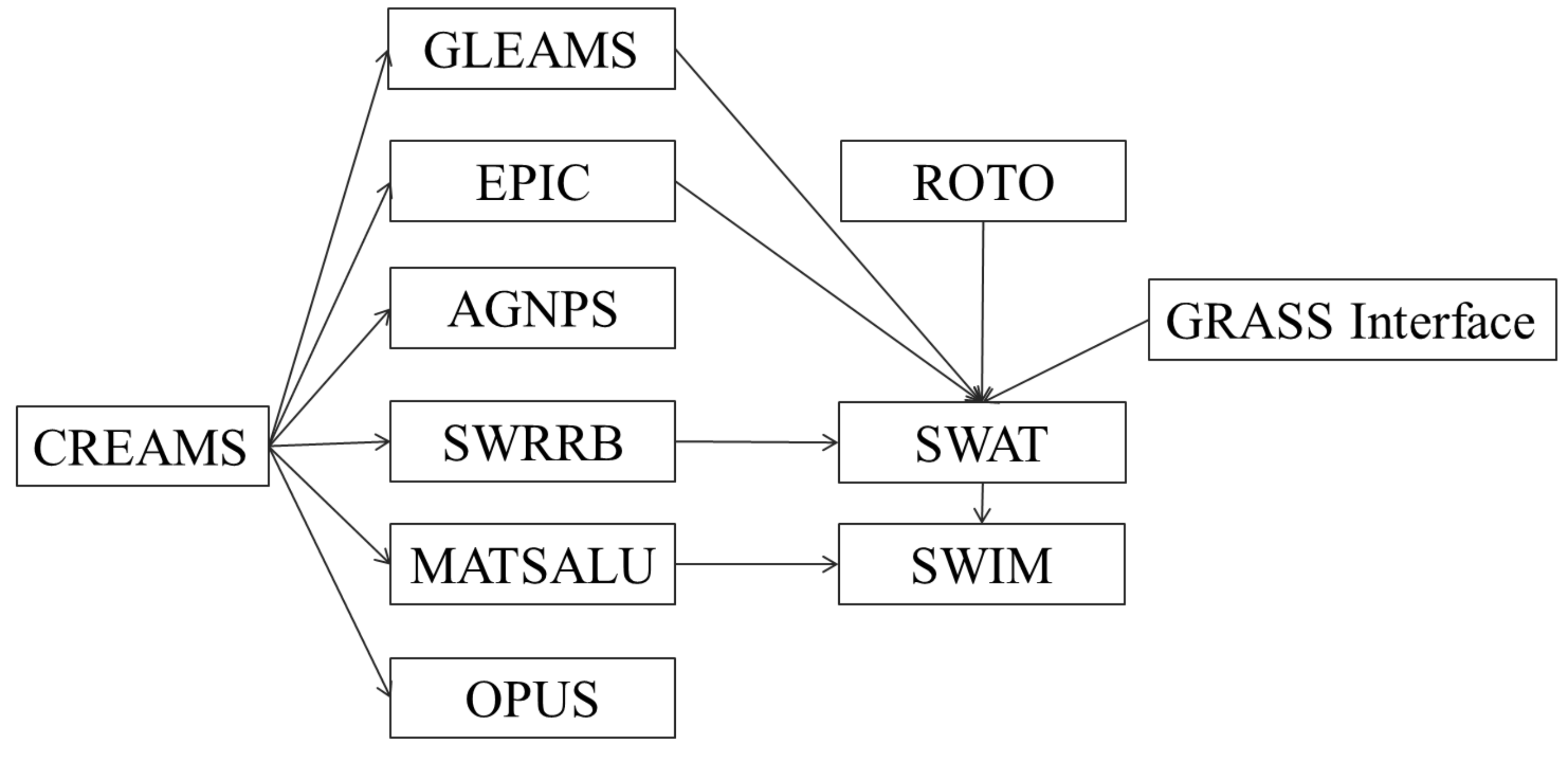
In the mid-1970’s in response to the Clean Water Act, the USDA Agricultural Research Service (ARS) assembled a team of interdisciplinary scientists to develop a process-based, nonpoint source simulation model. From that effort, a field scale model called CREAMS (Chemicals, Runoff, and Erosion from Agricultural Management Systems) was developed to simulate the impact of land management on water, sediment, and nutrients.
In the 1980’s, several models have been developed with origins from the CREAMS model. One of them, the GLEAMS model (Groundwater Loading Effects on Agricultural Management Systems) concentrated on pesticide and nutrient load to groundwater. Another model called EPIC (Erosion-Productivity Impact Calculator) was originally developed to simulate the impact of erosion on crop productivity and has now evolved into a comprehensive agricultural field scale model aimed in the assessment of agricultural management and nonpoint source loads. One more model for estimating the effects of different management practices on nonpoint source pollution from field-sized areas and also based on CREAMS is the OPUS model . These three models can be applied for the field-scale areas or small homogeneous watersheds.
Other efforts involved modifying CREAMS to simulate complex watersheds with varying soils, land use, and management, which resulted in the development of several models, like AGNPS , SWRRB and MATSALU .
AGNPS (AGricultural NonPoint Source) is a spatially detailed, single event (storm) model that subdivides complex watersheds into grid cells. SWRRB (Simulator for Water Resources in Rural Basins) was developed to simulate nonpoint source pollution from watersheds. It is a continuous time (daily time step) model that allows a basin to be subdivided into a maximum of ten sub-basins. To create SWRBB, the CREAMS model was modified for application to large, complex, rural basins.
The major changes involved were the following
the model was expanded to allow simultaneous computations on several sub-basins;
a better method was developed for predicting the peak runoff rate;
a lateral subsurface flow component was added;
a crop growth model was appended to account for annual variation in growth and its influence on hydrological processes;
a pond/reservoir storage component was adjoined;
a weather generator (rainfall, solar radiation, and temperature) was added for more representative weather inputs, both temporally and spatially;
a module accounting for transmission losses was appended;
a simple flood routing component was adjoined; and
a sediment routing component was added to simulate sediment movement through ponds, reservoirs, streams, and valleys.
SWRRB was still limited to ten sub-basins and had a simplistic routing structure with outputs routed from the sub-basin outlets directly to the basin outlet. This problem led to the development of a model called ROTO (Routing Outputs to Outlet) , which took outputs from SWRRB run on multiple sub-basins and routed the flows through channels and reservoirs. ROTO provided a reach routing approach and overcame the SWRRB sub-basin limitation by "linking" the sub-basin outputs.
Although the combination SWRRB + ROTO was quite effective, especially in comparison with CREAMS, the input and output of multiple files was cumbersome and required considerable computer storage. Limitations also occurred due to the fact that all SWRRB runs had to be made independently, and then the SWRRB outputs had to be input to ROTO for the channel and reservoir routing. Finally, the model called SWAT (Soil and Water Assessment Tool) was developed merging SWRRB and ROTO into one basin scale model. SWAT is a continuous time model working with daily time step, which allows a basin to be divided into hundreds or thousands of sub-watersheds or grid cells.
One more model, MATSALU, was developed in Estonia for the agricultural basin of the Matsalu Bay (which belongs to the Baltic Sea) with the area about 3,500 km2 and the bay ecosystem in order to evaluate different management scenarios for the eutrophication control of the Bay. The model consists of four coupled submodels, which simulate 1) watershed hydrology, 2) watershed geochemistry, 3) river transport of water and nutrients, and 4) nutrient dynamics in the Bay ecosystem. Similar to SWRRB, its watershed components were essentially based on the CREAMS approach.
Spatial disaggregation in MATSALU is based on the overlay of three map layers: a map of elementary watersheds with an average area of 10 km2, a land use map, and a soil map, to obtain so-called Elementary Areas of Pollution (EAP). Conceptually the EAPs are similar to Hydrologic Response Units (HRU) or hydrotopes. The three-level disaggregation scheme of MATSALU includes ‘the basin – elementary sub-basins – EAPs’. Since the model was developed for the MATSALU watershed and connected to specific data sets, it is not sufficiently transferable.
Merging the two tools: SWAT and MATSALU, we tried to keep their best features and maintain their advantages (see ). The model code was mostly based on SWAT. The more comprehensive three-level spatial disaggregation scheme from MATSALU was introduced into SWAT as an initial step. The next step was to adjust the model for the use in European conditions, where data availability is different. This required some efforts in order to modify the data input. Besides, several modules were excluded from SWAT (pesticides, ponds/reservoirs, lake water quality) in order to avoid the overparametrization.
[tbl:swat_matsalu_comparison]
| Advantages | Disadvantages | |
|---|---|---|
| SWAT |
|
|
| MATSALU |
|
|
In parallel to the model development, its modules were sequentially tested in the Elbe basin, starting from hydrology. In contrast to SWAT, the hydrological module of SWIM has been validated with a daily time step. During the test, some subroutines were modified, some parameters were changed, and some components have been substituted.
Currently the model SWIM includes some common (or similar) modules of both predecessors and some new routines, like the flow routing, which is based on Muskingum method instead of ROTO in SWAT and Sant-Venant approach in MATSALU. The SWAT/GRASS interface was modified for SWIM.
Further development of the model is planned in the following directions:
standardization of climate and crop management input data,
addition of a module accounting for the carbon cycle in soil;
addition of the lake and watershed modules;
improving the description of lateral transport of nutrients; and
modifying SWIM/GRASS interface to include automatic connection of climate/precipitation stations to sub-basins.
1.2 General Description
1.2.1 Model Objectives
The objectives of the model are two-fold:
to provide a comprehensive GIS-based tool for the coupled hydrological/ vegetation/water quality modelling in mesoscale watersheds (from 100 up to 10,000 km2), which can be parameterised using regionally available data, and
to enable the use of the model for analysis of climate change and land use change impacts on hydrological processes, agricultural production and water quality at the regional scale.
1.2.2 Processes Described in the Model
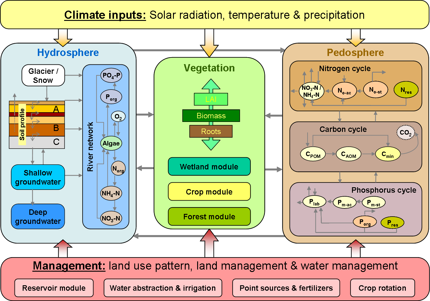
SWIM integrates hydrology, erosion, vegetation, and nitrogen/phosphorus dynamics at the river basin scale () and uses climate input data and agricultural management data as external forcing. The hydrological module is based on the water balance equation, taking into account precipitation, evapotranspiration, percolation, surface runoff, and subsurface runoff for the soil column subdivided into several layers.
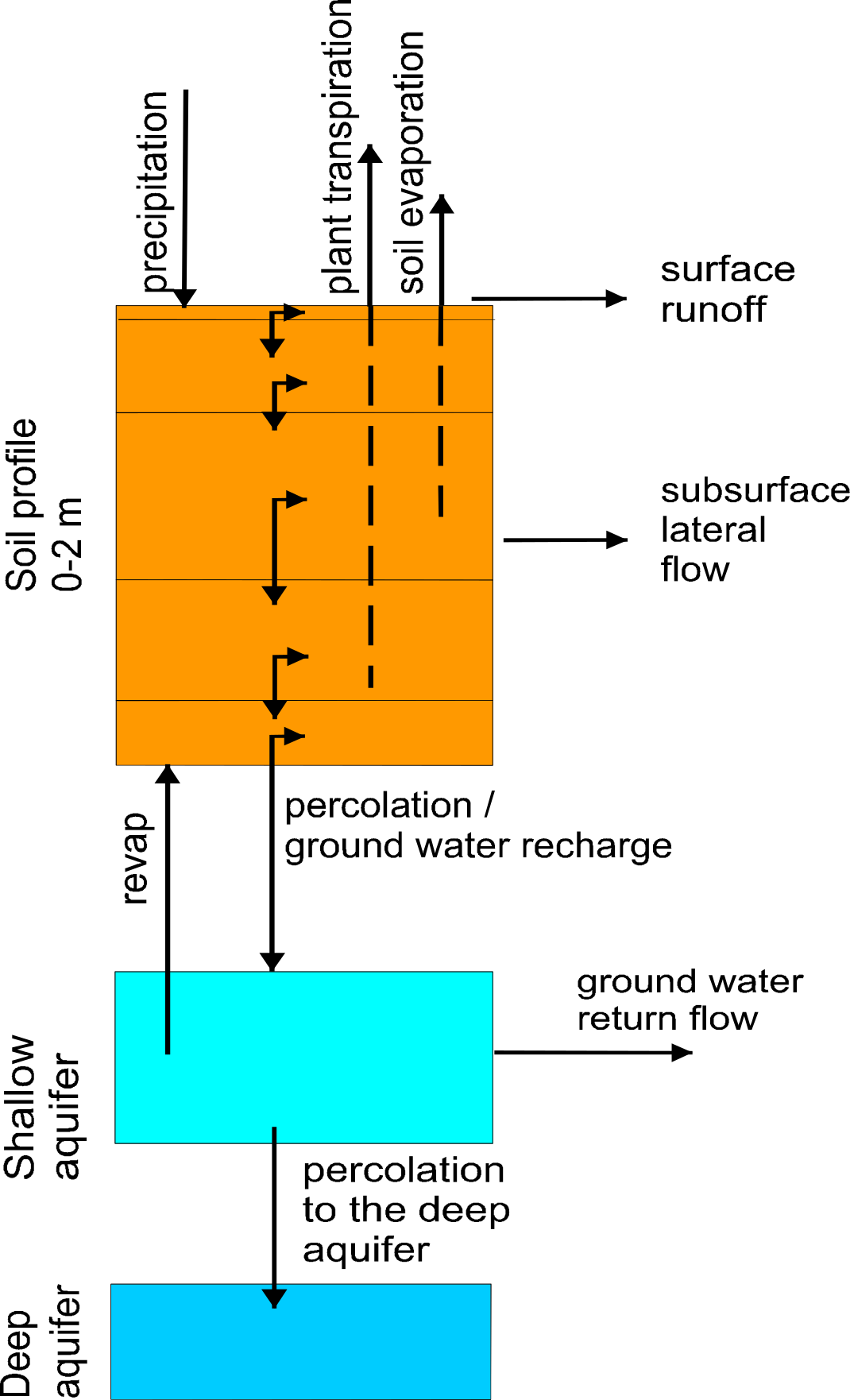
The simulated hydrological system consists of four control volumes: the soil surface, the root zone, the shallow aquifer, and the deep aquifer (). The percolation from the soil profile is assumed to recharge the shallow aquifer. Return flow from the shallow aquifer contributes to the streamflow. The soil column is subdivided into several layers in accordance with the soil data base. The water balance for the soil column includes precipitation, evapotranspiration, percolation, surface runoff, and subsurface runoff. The water balance for the shallow aquifer includes ground water recharge, capillary rise to the soil profile, lateral flow, and percolation to the deep aquifer.
[fig:soil_column_processes]
The nitrogen module includes the following pools (): nitrate nitrogen (NO3-N), active and stable organic nitrogen, organic nitrogen in the plant residue, and the flows: fertilisation, input with precipitation, mineralisation, denitrification, plant uptake, wash-off with surface and subsurface flows, leaching to ground water, and loss with erosion. The phosphorus module includes the pools: labile phosphorus, active and stable mineral phosphorus, organic phosphorus, and phosphorus in the plant residue, and the flows: fertilisation, sorption/desorption, mineralisation, plant uptake, loss with erosion, wash-off with lateral flow. The wash-off to surface water and leaching to groundwater are more important for nitrogen, while phosphorus is mainly transported with erosion.
[fig:nutrient_transport_scheme]
The module representing crop and natural vegetation is an important interface between hydrology and nutrients. The same as in SWAT, a simplified EPIC approach is included in SWIM for simulating all arable crops considered (wheat, barley, corn, potatoes, alfalfa, and others), using unique parameter values for each crop, which were obtained in different field studies. Simplification relates mainly to less detailed description of phenological processes and lower requirements on the input information. This enables to simulate crop growth in a distributed modelling framework for quite large basins and regions. Non-arable and natural vegetation is included in the database through some ‘aggregated’ vegetation types like ‘grass’, ‘pasture’, ‘forest’, etc. and can be simulated as well.
1.2.3 Spatial Disaggregation
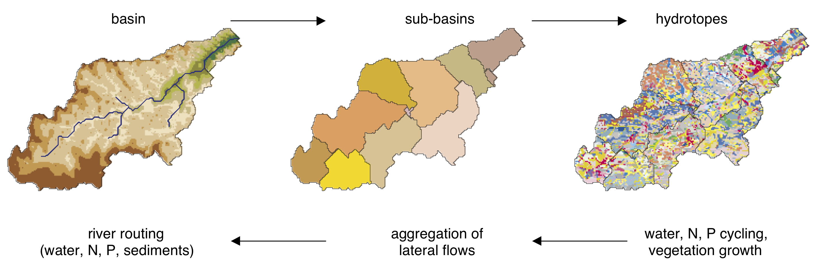
A three-level disaggregation scheme similar to that used in MATSALU is implemented in SWIM for mesoscale basins (). The three-level disaggregation scheme in SWIM implies 1) basin, 2) sub-basins, and 3) hydrotopes inside sub-basins.
[fig:spatial_disaggregation]
The idea is that a mesoscale basin (from 100 to 10,000 km2) is first subdivided into sub-basins of reasonable average area (see explanation in ). This can be done using the r.watershed program of GRASS (or any other GIS with similar capabilities), which is applied to a Digital Elevation Model of the area with a certain threshold for the average size of the sub-basin.
After that the hydrotopes (or HRUs) are delineated within every sub-basin, based on land use and soil types. Normally, a hydrotope is a set of disconnected units in the sub-basin, which have a unique land use and soil type. A hydrotope can be assumed to behave in a hydrologically uniform way within the sub-basin.
1.2.4 GIS Interface
The SWAT/GRASS interface was adopted and modified for SWIM to extract spatially distributed parameters of elevation, land use, soil types, and groundwater table. The interface creates a number of input files for the basin and sub-basins, including the hydrotope structure file (indicating sub-basin number, land use and soil type for every hydrotope) and the routing structure file (indicating how the sub-basins are connected via river network). To start the interface, the user must have at least four map layers of a basin. Three of them are the elevation map, the land use map, and the soil map. The fourth, sub-basin map, should be created in advance either using the r.watershed program of GRASS or by subdividing the basin in any other way.
- Step 1. Sub-basin attributes
This is the first step to be fulfilled. The program calculates area, resolution, and co-ordinate boundaries for the basin and each sub-basin, using a given sub-basin map. Further, the fraction of each sub-basin area to the basin area is calculated.
- Step 2. Topographic attributes
The program estimates the stream length, stream slope and geometrical dimensions using the r.stream.att tool . The cross sectional dimensions (width and depth) of a stream are estimated using a neural network that is embedded in the interface, based on the drainage area and average elevation of a sub-basin (which should be “trained” on the regional data before use). The accumulation area and aspect are computed using the standard methods in GRASS. The weighted average method is used to estimate the overland slope and slope length. Finally, the channel USLE (Universal Soil Loss Equation) factors K and C are estimated using a standard table.
- Step 3. Hydrotope structure
The program defines the basin hydrotope structure by overlaying the sub-basin map with land use and soil layers. The structure file is created to run the model. Each line in the file describes the characteristics of one hydrotope - its sub-basin number, land use, and soil.
- Step 4. Weather attributes
The program selects the closest weather/precipitation station to every sub-basin. Then either actual weather information can be used, or the weather generator (in this case the long-term monthly statistical parameters must be available for precipitation and temperature for the station). This part of the interface has to be modified to provide more flexible input of climate information.
- Step 5. Ground water attributes
The ground water parameters are estimated for each sub-basin using the alpha layer (the reaction factor described in ). This parameter defines the time lag needed to the groundwater flow as it leaves the shallow aquifer to reach the stream.
- Step 6. Routing structure
The interface creates the routing structure for the basin based on the elevation map. The routing structure is put in a special file, which provides the information about when to add flows and route through sub-basins and when to add inflow (or subtract withdrawals) from any sub-basins.
Steps 1, 2, 5, 6 described above are the same as in the SWAT/GRASS interface, steps 3 and 4 are new, and some other steps from SWAT/GRASS (such as irrigation and nutrient attributes) were excluded.
1.2.5 Modelling Procedure
First, the SWIM/GRASS interface runs to produce necessary input files. After that the model itself can be run. The model operates on a daily time step. After the input parameters are read from files, the three-step modelling procedure is applied. First, water and nitrogen dynamics and crop/vegetation growth are calculated for every hydrotope. Then the outputs from the hydrotopes, especially the lateral water and nutrient flows, are averaged (area-weighted average) to estimate the sub-basin output. Finally, the routing procedure is applied to the sub-basin outputs, taking transmission losses into account.
1.3 Overview of the Model Components
1.3.1 Hydrological Processes
Snow melt The snow melt component is similar to that of the CREAMS model , according to a simple degree-day equation. Melted snow is then treated in the same way as rainfall for further estimation of runoff and percolation.
Surface runoff The runoff volume is estimated using a modification of the SCS curve number method . Surface runoff is predicted as a nonlinear function of precipitation and a retention coefficient. The latter depends on soil water content, land use, soil type, and management. The curve number and the retention coefficient vary non-linearly from dry conditions at wilting point to wet conditions at field capacity and approach 100 and 0 respectively at saturation. The modification essentially reduced the empirism of the original curve number method. The reliability of the method has been proven by multiple validation of SWAT and SWIM in mesoscale basins. Nevertheless, there is a possibility to exclude the dependence of the retention coefficient on land use and soil, leaving the dependence on soil water content only, and assuming the same interval for all types of land use and soils.
Percolation The same storage routing technique as in SWAT is used to simulate water flow through soil layers in the root zone. Downward flow occurs when field capacity of the soil layer is exceeded, and as long as the layer below is not saturated. The flow rate is governed by the saturated hydraulic conductivity of the soil layer. Once water percolates below the root zone, it becomes groundwater. Since the one day time interval is relatively large for soil water routing, the inflow is divided into 4 mm slugs in order to take into account the flow rate’s dependence on soil water content. If the soil temperature in a layer is below 0°C, no percolation occurs from that layer. The soil temperature is estimated for each soil layer using the air temperature as a driver .
Lateral subsurface flow Lateral subsurface flow is calculated simultaneously with percolation. The kinematic storage model developed by is used to estimate the subsurface flow. The approach is based on the mass continuity equation in the finite difference form with the entire soil profile as the control volume. To account for multiple layers, the model is applied to each soil layer independently starting at the upper layer to allow for percolation from one soil layer to the next and percolation from the bottom soil layer past the soil profile (as recharge to the shallow aquifer).
Evapotranspiration Potential evapotranspiration is estimated using the Priestley-Taylor method (1972) that requires solar radiation and air temperature as input. It is possible to use the Penman-Monteith method instead if wind speed and relative air humidity data can be provided in addition. The actual evapotranspiration is estimated following the concept, separately for soil and plants. Actual soil evaporation is computed in two stages. It is equal to the potential soil evaporation predicted by means of an exponential function of leaf area index until the accumulated soil evaporation exceeds the upper limit of 6 mm. After that stage two begins. The actual soil evaporation is reduced and estimated as a function of the number of days since stage two began. Plant transpiration is simulated as a linear function of potential evapotranspiration and leaf area index. When soil water is limited, plant transpiration is reduced, taking into account the root depth.
Groundwater flow The groundwater model component is the same as in SWAT (see . The percolation from the soil profile is assumed to recharge the shallow aquifer. Return flow from the shallow aquifer contributes directly to the streamflow. The equation for return flow was derived from , assuming that the variation in return flow is linearly related to the rate of change of the water table height. In a finite difference form, the return flow is a nonlinear function of ground water recharge and the reaction factor RF, the latter being a direct index of the intensity with which the groundwater outflow responds to changes in recharge. The reaction factor can be estimated for gaged sub-basins using the base flow recession curve.
1.3.2 Crop / Vegetation Growth
The crop model in SWIM and SWAT is a simplification of the EPIC crop model . The SWIM model uses a concept of phenological crop development based on
daily accumulated heat units;
Monteith’s approach (1977) for potential biomass;
water, temperature, and nutrients stress factors; and
harvest index for partitioning grain yield.
However, the more detailed approach implemented in EPIC for the root growth and nutrient cycling is not included in order to maintain a similar level of complexity of all submodels and to keep control on the model performance.
A single model is used for simulating all the crops and natural vegetation included in the crop database attached to the model. Annual crops grow from planting date to harvest date or until the accumulated heat units reach the potential heat units for the crop. Perennial crops maintain their root systems throughout the year, although the plants may become dormant after frost.
Phenological development of the crop is based on daily heat unit accumulation. Interception of photosynthetic active radiation is estimated with Beer’s law equation as a function of solar radiation and leaf area index. The potential increase in biomass is the product of absorbed PAR and a specific plant parameter for converting energy into biomass.
The potential biomass is adjusted daily if one of the four plant stress factors (water, temperature, nitrogen, and phosphorus) is less than 1.0 using the product of a minimum stress factor and the potential biomass. The water stress factor is defined as the ratio of actual to potential plant transpiration. The temperature stress factor is computed as a function of daily average temperature, optimal and base temperatures for plant growth. The N and P stress factors are based on the ratio of accumulated N and P to the optimal values.
The fraction of daily biomass growth partitioned to roots is estimated to range linearly between two fractions specified for each vegetation type - 0.4 at emergence to 0.2 at maturity. Root depth increases as a linear function of heat units and potential root depth. Leaf area index is simulated as a nonlinear function of accumulated heat units and crop development stages. Crop yield is estimated using the harvest index, which increases as a nonlinear function of heat units from zero at planting to the optimal value at maturity. The harvest index is affected by water stress in the second half of the growing period.
1.3.3 Nutrient Dynamics
Nitrogen mineralisation The nitrogen mineralisation model is a modification of the PAPRAN mineralisation model (Seligman and van Keulen, 1981). Organic nitrogen associated with humus is divided into two pools: active or readily mineralisable organic nitrogen and stable organic nitrogen. The model considers two sources of mineralisation: a) fresh organic nitrogen pool, associated with crop residue, and b) the active organic nitrogen pool, associated with the soil humus. Organic N flow between the active and stable organic nitrogen pools is governed by the equilibrium equation. Mineralisation of fresh organic nitrogen is a function of the C:N ratio, C:P ratio, soil temperature, and soil water content. The N mineralisation flow from residue is distributed between the mineral nitrogen (80%) and active organic nitrogen (20%) pools. Mineralisation of the active organic nitrogen pool depends on soil temperature and water content.
Phosphorus mineralization The phosphorus mineralisation model is structurally similar to the nitrogen mineralisation model. To maintain phosphorus balance at the end of a day, humus mineralisation is subtracted from the organic phosphorus pool and added to the mineral phosphorus pool, and residue mineralisation is distributed between the organic phosphorus pool (20%) and the labile phosphorus (80%).
Sorption / adsorption of phosphorus Mineral phosphorus is distributed between three pools: labile phosphorus, active mineral phosphorus, and stabile mineral phosphorus. Mineral phosphorus flow between the active and stable mineral pools is governed by the equilibrium equation, assuming that the stable mineral pool is four times larger. Mineral phosphorus flow between the active and labile mineral pools is governed by the equilibrium equation as well, assuming equal distribution.
Denitrification Denitrification, as one of the microbial processes, is a function of temperature and water content. The denitrification occurs only in the conditions of oxygen deficit, which usually takes place when soil is wet. The denitrification rate is estimated as a function of soil water content, soil temperature, organic matter, a coefficient of soil wetness, and mineral nitrogen content. The soil water factor is an exponential function of soil moisture with an increasing trend when soil becomes wet.
Crop uptake of nutrients Crop uptake of nitrogen and phosphorus is estimated using a supply and demand approach. Six parameters are specified for every crop in the crop database, which describe: BN1 and BP1 - normal fraction of nitrogen and phosphorus in plant biomass excluding seed at emergence, BN2 and BP2 – at 0.5 maturity, and BN3 and BP3 - at maturity. Then the optimal crop N and P concentrations are calculated as functions of growth stage. The daily crop demand of nutrients is estimated as the product of biomass growth and optimal concentration in the plants. Actual nitrogen and phosphorus uptake is the minimum of supply and demand. The crop is allowed to take nutrients from any soil layer that has roots. Uptake starts at the upper layer and proceeds downward until the daily demand is met or until all nutrient content has been depleted.
Soluble nutrient loss in surface water and groundwater The amount of NO3-N and soluble P in surface runoff is estimated considering the top soil layer only. Amounts of NO3-N and soluble P in surface runoff, lateral subsurface flow and percolation are estimated as the products of the volume of water and the average concentration. Retention factor is taken into account through transmission losses. Because phosphorus is mostly associated with the sediment phase, the soluble phosphorus loss is estimated as a function of surface runoff and the concentration of labile phosphorus in the top soil layer.
1.3.4 Erosion
Sediment yield is calculated for each sub-basin with the Modified Universal Soil Loss Equation (MUSLE, ), almost the same as in SWAT. The equation for sediment yield includes the runoff factor, the soil erodibility factor, the crop management factor, the erosion control practice factor, and the slope length and steepness factor. The only difference from SWAT is that the surface runoff, the soil erodibility factor and the crop management factor are estimated for every hydrotope, and then averaged for the sub-basin (weighted areal average).
Estimation of the runoff factor requires the characteristics of rainfall intensity as described in . To estimate the daily rainfall energy in the absence of time-distributed rainfall, the assumption about exponential distribution of the rainfall rate is made. This stochastic element is included to allow more realistic representation of peak runoff rates, given only daily rainfall and monthly rainfall intensity. This allows a simple substitution of rainfall rates into the equation. The fraction of rainfall that occurs during 0.5 hours is simulated stochastically, taking into account average monthly rainfall intensity for the area. Soil erodibility factor can be estimated from the texture of the upper soil layer. The slope length and steepness factor is estimated based on the Digital Elevation Model of a watershed by SWIM/GRASS interface for every sub-basin.
1.3.5 River Routing
The Muskingum flow routing method is used in SWIM. The Muskingum equation is derived from the finite difference form of the continuity equation and the variable discharge storage equation. The outflow rate for the reach is estimated using a requrrent equation with two parameters. They are the storage time constant for the reach, KST, and a dimensionless weighting factor, X. In physical terms, the parameter KST corresponds to an average reach travel time, and X indicates the relative importance of the inflow and outflow in determining the storage in the reach.
The sediment routing model consists of two components operating simultaneously – deposition and degradation in the streams. The approach is based on the estimation of the stream velocity in the channel as a function of the peak flow rate, the flow depth, and the average channel width. The sediment delivery ratio is estimated using a power function (power 1 to 1.5) of the stream velocity. If the sediment delivery ratio is less than 1, the deposition occurs in the stream, and degradation is zero. Otherwise, degradation is estimated as a function of the sediment delivery ratio, the channel K factor (or the effective hydraulic conductivity of the channel alluvium), and the channel C factor.
Nitrate nitrogen and soluble phosphorus are considered in the model as conservative materials for the duration of an individual runoff event . Thus they are routed by adding contributions from all sub-basins to determine the basin load.
2 Mathematical Description of the Model Components
In this chapter a mathematical description of all model components is given. First, hydrological processes are described in , followed by vegetation/crop growth processes (), nutrient dynamics processes (), and erosion (). After that a description of the channel routing processes is given in . This chapter is based mostly on the SWAT User Manual and the MATSALU model description .
2.1 Hydrological Processes
The hydrological submodel in SWIM is based on the following water balance equation \[\label{eq:hydrological_processes} SW(t + 1) = SW(t)+ PRECIP -Q - ET - PERC - SSF\]
where SW(t) is the soil water content in the day t, PRECIP – precipitation, Q – surface runoff, ET - evapotranspiration, PERC - percolation, and SSF – subsurface flow. All values are the daily amounts in mm. Here the precipitation is an input, assuming that precipitation may differ between sub-basins, but it is uniformly distributed inside the subbasin. The melted snow is added to precipitation. The surface runoff, evapotranspiration, percolation below root zone and subsurface flow are described below. Some river basins, especially in the semiarid zone, have alluvial channels that abstract large quantities of stream flow. The transmission losses reduce runoff volumes when the flood wave travels downstream. This reduction is taken into account by a special module that accounts for transmission losses.
2.1.1 Snow Melt
If air temperature is below 0, precipitation occurs as snow, and snow is accumulated. If snow is present on soil, it may be melted when the temperature of the second soil layer exceeds 0°C (according to the model requirements, the depth of the first soil layer must be always set to 10 mm). The approach used is similar to that of CREAMS model . Snow is melted as a function of the snow pack temperature in accordance with the equation
\[\label{eq:snow_melt} \begin{array}{c} SML=4.57*TMX \\ 0. \leq \ SML \leq \ SNO \end{array}\]
where SML is the snowmelt rate in mm d-1, SNO is the snow in mm of water, TMX is the maximum daily air temperature in °C. Melted snow is treated the same as rainfall for estimating runoff volume and percolation, but rainfall energy is set to 0.
2.1.2 Surface Runoff
The model takes the daily rainfall amounts as input and simulates surface runoff volumes and peak runoff rates. Runoff volume is estimated by using a modification of the Soil Conservation Service (SCS) curve number technique . The technique was selected for use in SWIM as well as in SWAT due to several reasons:
(a) it is reliable and has been used for many years in the United States and worldwide;
(b) the required inputs are usually available;
(c) it relates runoff to soil type, land use, and management practices; and
(d) it is computationally efficient.
The use of daily precipitation data is a particularly important feature of the technique because for many locations, and especially at the regional scale, more detailed precipitation data with time increments of less than one day are not available. Surface runoff is estimated from daily precipitation taking into account a dynamic retention coefficient SMX by using the SCS curve number equation
\[\label{eq:SCS_curve_number} \begin{array}{c} Q=\frac{(PRECIP - 0.2 * SMX)^2}{(PRECIP + 0.8 * SMX)},\quad PRECIP > 0.2*SMX \\ Q=0,\quad PRECIP \leq \ 0.2 * SMX \end{array}\]
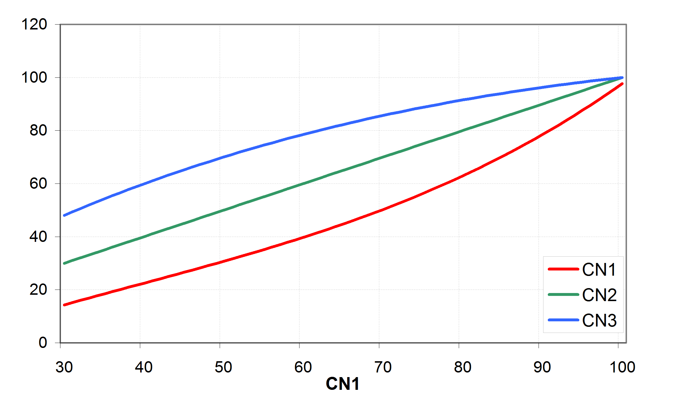
where Q is the daily runoff in mm, PRECIP is the daily precipitation in mm, and SMX is a retention coefficient. The retention coefficient SMX varies a) spatially, because soils, land use, management, and slope vary, and b) temporally, because soil water content is changing. The retention coefficient SMX is related to the curve number CN by the SCS equation
\[\label{eq:SMX_retention_coefficient} SMX = 254 *\biggl(\frac{100}{CN}-1\biggl)\]
To illustrate the approach, shows estimation of surface runoff Q from daily precipitation with () and () assuming different CN values.

The parameter CN is defined in three variations:
· for moisture condition 1 (or dry conditions) as CN1
· for moisture condition 2 (or average conditions) as CN2 and
· for moisture condition 3 (or wet conditions) as CN3.
CN2 can be obtained from the SCS hydrology handbook for a set of land use types, hydrologic soil groups and management practices (see also Tab. 3.20 in of the Manual). The corresponding values of CN1 and CN3 are also tabulated in the handbook. For computing purposes, CN1 and CN3 were related to CN2 with the equations (see also ) \[\label{eq:Surface_Runoff5}
CN\textsubscript{1}=CN\textsubscript{2}- \frac{20* (100- CN\textsubscript{2})}{100 - CN\textsubscript{2}+ exp\biggl[2.533 - 0.0636 * (100-CN\textsubscript{2})\biggl]}\]
or an approximation of : \[\label{eq:Surface_Runoff6} CN\textsubscript{1}= -16.911 + 1.3481 * CN\textsubscript{2} - 0.013793 * CN\textsubscript{2}\textsuperscript{2} + 0.00011772 * CN\textsubscript{2}\textsuperscript{3}\] and \[\label{eq:Surface_Runoff7} CN\textsubscript{3}= CN\textsubscript{2} * exp\biggl[0.00673 * (100 - CN\textsubscript{2})\biggl]\]
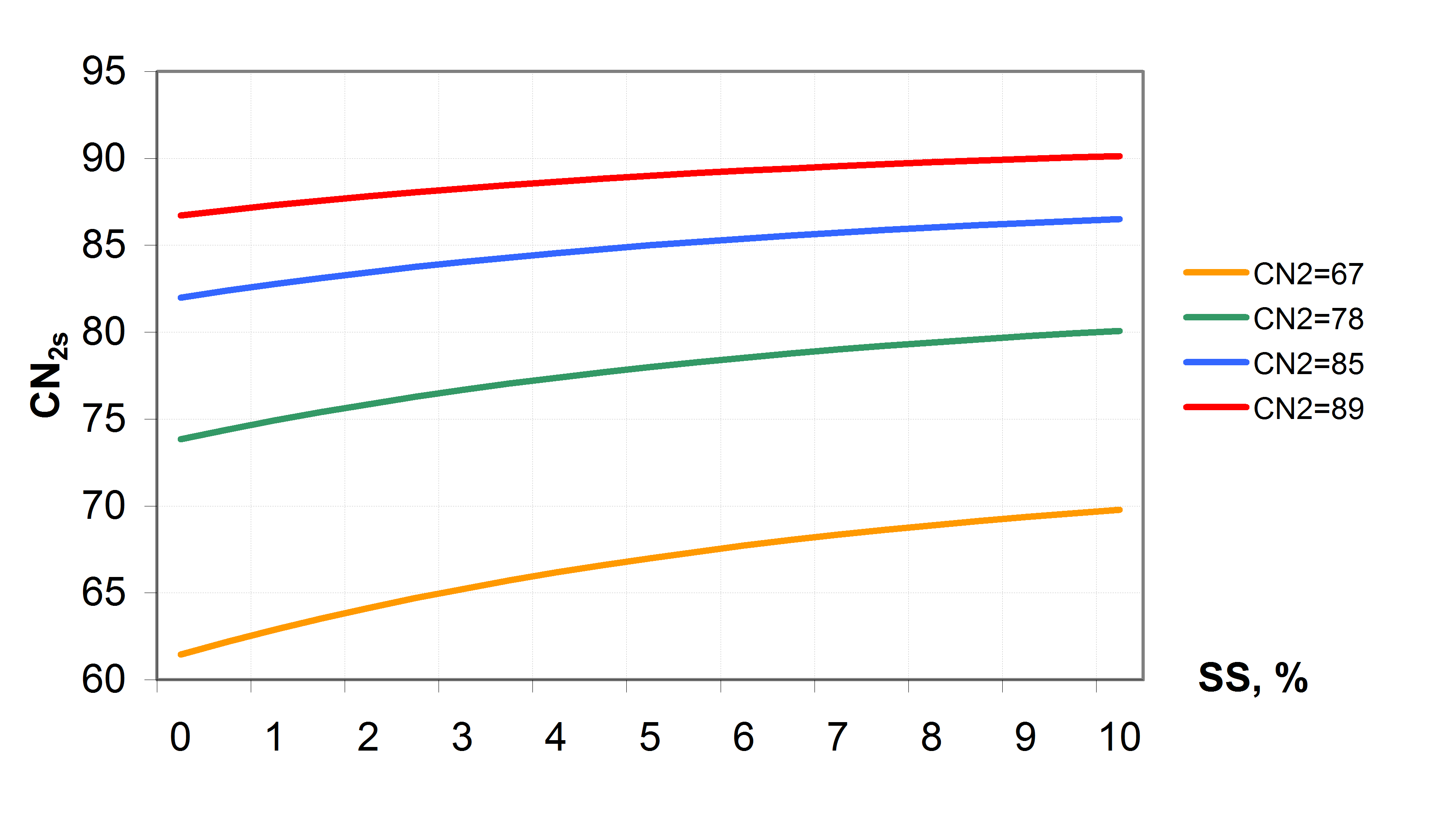
The values of CN1, CN2 and CN3 are related to land use types, hydrologic soil groups and management practices. An additional assumption was made to relate curve numbers to slope. Namely, it was assumed that the CN2 value is appropriate for a 5% slope, the following equation was derived to adjust it for lower and higher slopes (see also ): \[\label{eq:Surface_Runoff8} CN\textsubscript{2}\textsubscript{S}= CN\textsubscript{2} + \frac{CN\textsubscript{3}- CN\textsubscript{2}}{3}* (1-2*exp(-13.86 * SS))\] where CN2S is the adjusted CN2 value, and SS is the slope steepness in m m-1. The retention coefficient is changing dynamically due to fluctuations in soil water content according to the equation \[\label{eq:Surface_Runoff9} SMX = SMX\textsubscript{1} *\biggl(1- \frac{SW}{SW + exp(WF\textsubscript{1}- WF\textsubscript{2}*SW)}\biggl)\] where SMX1 is the value of SMX associated with CN1, SW is the soil water content in mm, and WF1 and WF2 are shape parameters. depicts the relationships between the retention coefficient SMX and the curve number CN, on one hand, and the relative soil water content, on the other hand.
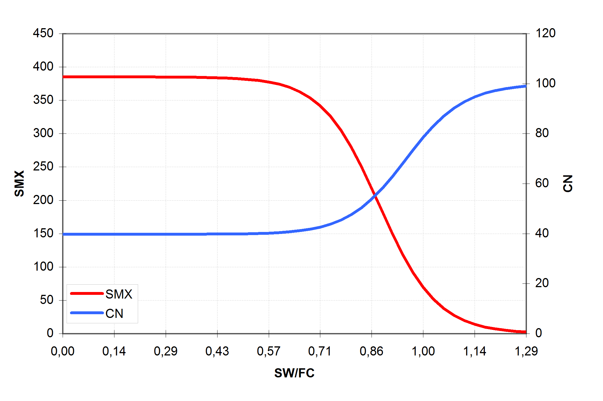
The following assumptions are made for the retention coefficient SMX \[\label{eq:Surface_Runoff10}
\begin{array}{c}
SMX=SMX\textsubscript{1} \qquad if SW=WP, \\
SMX=SMX\textsubscript{2} \qquad if FCC=0.7, \\
SMX=SMX\textsubscript{3} \qquad if SW=FC, \\
SMX=2.54 \qquad if SW=PO
\end{array}\] where SMX2 is the retention parameter corresponding to CN2, SMX3 is the retention parameter corresponding to CN3, WP is the wilting point water content in mm mm-1, FC is the field capacity water content in mm mm-1, PO is the soil porosity in mm mm-1, and FFC is the fraction of field capacity defined with the equation \[\label{Surface_Runoff11}
FFC= \frac{SW-WP}{FC-WP}\] The assumption that SMX = 2.54 in () means that at full saturation CN = 99 (approaches its maximum). Values for WF1 and WF2 are obtained from a simultaneous solution of according to the assumptions () as following \[WF\textsubscript{1}=ln\biggl(\frac{FC}{1-SMX\textsubscript{3}/SMX\textsubscript{1}}-FC\biggl)+FC*WF\textsubscript{2}\] \[WF\textsubscript{2}=\frac{ln\biggl(\frac{FC}{1-SMX\textsubscript{3}/SMX\textsubscript{1}}-FC\biggl)-ln\biggl(\frac{PO}{1-2.54/SMX\textsubscript{1}}-PO\biggl)}{PO-FC}\] The value of FFC defined in represents soil water uniformly distributed through the root zone of soil or the upper 1m of soil. Runoff estimates can be improved if the depth distribution of water in soil is known. For example, water distributed near the soil surface results in more runoff than the same volume of water uniformly distributed throughout the soil profile. Since SWIM estimates water content of each soil layer daily, the depth distribution is available. The effect of depth distribution on runoff is expressed in the depth weighting function \[FFC\textsuperscript{*}=\frac{\sum\nolimits_{i=1}^M\biggl(FFC\textsubscript{i}*\frac{Z\textsubscript{i}-Z\textsubscript{i-1}}{Z\textsubscript{i}}\biggl)}{\sum\nolimits_{i=1}^M\biggl(\frac{Z\textsubscript{i}-Z\textsubscript{i-1}}{Z\textsubscript{i}}\biggl)}, \qquad Z\textsubscript{1}\leq1.0m\] where FFC* is the depth-weighted FFC value for use in (), Zi is the depth to the bottom of soil layer i in mm, and M is the number of soil layers. Equation 14 performs two functions:
a) it reduces the influence of lower layers because FFCi is divided by Zi and
b) it gives proper weight to thick layers relative to thin layers because FFC is multiplied by the layer thickness.
There is also a possibility for estimating runoff from frozen soil. If the temperature of the second soil layer is less than 0°C, the retention coefficient is reduced by using the equation \[\label{eq:Surface_Runoff15}
SMX\textsubscript{froz}=SMX*\biggl(1.-exp(-0.000862 * SMX)\biggl)\] where SMXfroz is the retention coefficient for frozen ground. increases runoff for frozen soils, but allows significant infiltration when soil is dry.
2.1.3 Peak Runoff Rate
The peak runoff rate is estimated in SWIM for sub-basins using the modified Rational formula . A stochastic element is included in the Rational formula to allow a more realistic simulation of peak runoff rates, given only daily rainfall and monthly rainfall intensity. The Rational formula can be written in the form \[\label{eq:Surface_Runoff16}
PEAKQ=\frac{RUNC * RI * A}{360}\] where PEAKQ is the peak runoff rate in m³ s-1, RUNC is a dimentionless runoff coefficient expressing the watershed infiltration characteristics, RI is the rainfall intensity in mm h-1 for the watershed’s time of concentration, and A is the drainage area in ha.
The runoff coefficient can be calculated for each day from the amounts of precipitation and runoff as following \[\label{eq:Surface_Runoff17}
RUNC= \frac{Q}{PRECIP}\] Since daily precipitation is input and Q is calculated with , RUNC can be estimated directly.
Rainfall intensity can be expressed as \[\label{eq:Surface_Runoff18}
RI=\frac{PERCIP\textsubscript{tC}}{TC}\] where TC is the watershed’s time of concentration in h, and PRECIPtC is the amount of rainfall in mm during the time of concentration.
The value of PRECIPtC can be estimated by developing a relationship with total daily PRECIP. Generally, PRECIPtc and PRECIP24 (24-h duration is appropriate for the daily time step model) are proportional for various frequencies.
Thus, a dimensionless parameter a that expresses the proportion of total daily rainfall that occurs during time of concentration can be introduced. Then \[\label{eq:Surface_Runoff19}
PRECIP\textsubscript{tC}=\alpha*PRECIP\textsubscript{24}\] The equation for the peak runoff rate is obtained by substituting , , and into : \[PEAKQ=\frac{\alpha*Q*A}{360*TC}\] The time of concentration can be estimated by adding the surface and channel flow times \[TC=TC\textsubscript{ch}+ TC\textsubscript{ov}\] where TCch is the time of concentration for channel flow in h, and TCov is the time of concentration for overland surface flow in h.
The time of concentration for channel flow can be calculated by the equation \[TC\textsubscript{ch}=\frac{CHFL}{3.6 * CHV}\] where CHFL is the average channel flow length for the basin in km and CHV is the average channel velocity in m s-1.
The average channel flow length can be estimated by the equation \[CHFL=\sqrt{CHL * CHL\textsubscript{cen}}\] where CHL is the channel length from the most distant point to the watershed outlet in km and CHLcen is the distance from the outlet along the channel to the watershed centroid in km. We can assume that CHLcen=0.5 CHL.
Average velocity can be estimated by using Manning’s equation and assuming a trapezoidal channel with 2:1 side slopes and a 10:1 bottom width to depth ratio. Substitution of these estimated and assumed values, and conversion of units gives the following estimation of the time of concentration for channel \[TC\textsubscript{ch}=\frac{0.62 * CHL * CHN\textsuperscript{0.75}}{(QAV * A)\textsuperscript{0.25}* CHS\textsuperscript{0.375}}\] where CHN is Manning’s n, QAV is the average flow rate in mm h-1, and CHS is the average channel slope in m m-1.
The average flow rate is obtained from the estimated average flow rate from a unit source in the watershed (1 ha area) and the relationship \[QAV= QAV\textsubscript{0}* A\textsuperscript{-0.5}\] where QAV0 is the average flow rate from a 1 ha area in mm h-1.
Substitution of equation 25 into equation 24 gives the final equation for TCch: \[TC\textsubscript{ch}=\frac{0.62 * CHL * CHN\textsuperscript{0.75}}{QAV\textsubscript{0}\textsuperscript{0.25}*A\textsuperscript{0.125}* CHS\textsuperscript{0.375}}\] A similar approach is used to estimate the time of concentration for overland surface flow \[\label{eq:Surface_Runoff27}
TC\textsubscript{ov}=\frac{SL}{3600 * SV}\] where SL is the surface slope length in m and SV is the surface flow velocity in m s-1.
The surface flow velocity is estimated applying Manning’s equation to a strip 1 m wide down the slope length, and assuming that flow is concentrated into a small trapezoidal channel with 1:1 side slopes and 5:1 bottom width to depth ratio as following
\[\label{eq:Surface_Runoff28} SV= \frac{0.00748 * FD\textsuperscript{0.666}*SS\textsuperscript{0.5}}{SN}\]
where SV is the surface flow velocity in m³ s-1, FD is flow depth in m, SS is the land surface slope in m m-1, and SN is Manning’s roughness coefficient ‘n’ for the surface.
The average flow depth FD is calculated from Manning’s equation as a function of flow rate
\[\label{eq:Surface_Runoff29} FD=\biggl(\frac{QAV\textsubscript{0}*SN}{5.025 * SS\textsuperscript{0.5}}\biggl)\textsuperscript{0.375}\]
where AVQ0 is the average flow rate in m³ s-1. Substitution of equations and into gives
\[TC\textsubscript{ov}=\frac{0.0556 * SL * SN\textsuperscript{0.75}}{QAV\textsubscript{0}\textsuperscript{0.25}*SS\textsuperscript{0.375}}\]
The average flow rate from a unit source area in the basin is estimated with the equation
\[QAV\textsubscript{0}=\frac{Q}{DUR}\]
where the rainfall duration DUR (in h) is calculated using the equation
\[\label{eq:Surface_Runoff32} DUR= \frac{2.303}{-ln(1.-\alpha\textsubscript{0.5})}\]
where \(\alpha\textsubscript{0.5}\) is the fraction of rainfall that occurs during 0.5 h. It is calculated with using PRECIP0.5 instead of PRECIPtC.
is derived assuming that rainfall intensity is exponentially distributed. To evaluate \(\alpha\) properly, variation in rainfall patterns must be considered. For some short duration storms, most or all the rain occurs during TC causing \(\alpha\) to approach its upper limit of 1.0. Other storm events of uniform intensity cause \(\alpha\) to approach a minimum value. By substituting the products of intensity and time into , an expression for the minimum value of \(\alpha\), \(\alpha\textsubscript{min}\), is obtained
\[\alpha\textsubscript{min}=TC/24\]
Thus, \(\alpha\) ranges within the limits
\[TC/24<\alpha<1.0\]
Although confined between limits, the value of \(\alpha\) is assigned with considerable uncertainty when only daily rainfall and simulated runoff amounts are given. This can lead to considerable uncertainties in estimating daily runoff and has to be kept in mind. The value of \(\alpha\) is estimated in the model from the gamma distribution, taking into account the average monthly rainfall intensity for the basin under study.
2.1.4 Percolation
A storage routing technique is used in SWIM to simulate percolation through each soil layer. The percolation from the bottom soil layer is treated as recharge to the shallow aquifer. The storage routing technique is based on the equation
\[SW(t+1) =SW(t) * exp\biggl(\frac{-\Delta t}{TT\textsubscript{i}}\biggl)\]
where SW(t+1) and SW(t) are the soil water contents at the beginning and end of the day in mm, Dt is the time interval (24 h), and TTi is the travel time through layer i in h. Thus, the percolation can be calculated by subtracting SWt from SWt+1:
\[\label{eq:Percolation36} PERC\textsubscript{i}=SW\textsubscript{i}*\biggl[1. - exp\biggl(\frac{-\Delta t}{TT\textsubscript{i}}\biggl)\biggl]\]
where PERC is the percolation rate in mm d-1. The travel time TTi is calculated for each soil layer with the linear storage equation
\[\label{eq:Percolation37} TT\textsubscript{i}= \frac{SW\textsubscript{i} - FC\textsubscript{i}}{HC\textsubscript{i}}\]
where HCi is the hydraulic conductivity in mm h-1 and FC is the field capacity water content for layer i in mm. The hydraulic conductivity is varying from the saturated conductivity value at saturation to near zero at field capacity (see also ) as
\[\label{eq:Percolation38} HC\textsubscript{i}= SC\textsubscript{i}* \biggl(\frac{SW\textsubscript{i}}{UL\textsubscript{i}}\biggl)\textsuperscript{$\beta\textsubscript{i}$}\]
where SCi is the saturated conductivity for layer i in mm h-1, ULi is soil water content at saturation in mm mm-1, and \(\beta\)i is a shape parameter that causes HCi to approach zero as SWi approaches FCi. The equation for estimating \(\beta\)i is
\[\label{eq:Percolation39} \beta\textsubscript{i}= \frac{-2.655}{log\textsubscript{10}(\frac{FC\textsubscript{i}}{UL\textsubscript{i}})}\]

The constant in equation 39 is set to –2.655 to assure that at field capacity
\[\label{eq:Percolation40} HC\textsubscript{i}=0.002 * SC\textsubscript{i}\]
Water flow through a soil layer may occur until the lower layer is not saturated. If the layer below the layer being considered is saturated, no flow can occur. The effect of lower layer water content is expressed by the equation
\[\label{eq:Percolation41} PERC\textsubscript{ic}= PERC\textsubscript{i}* \sqrt{1 - \frac{SW\textsubscript{i}+ 1}{UL\textsubscript{i}+1}}\]
where PERCic is the percolation rate for layer i in mm d-1 corrected for layer i+1 water content and PERCi is the percolation calculated with .
Percolation is also affected by soil temperature. If the temperature in a particular layer is O°C or below, no percolation is allowed from that layer.
Since the one-day time interval is relatively low for routing flow through the soil root zone, the water is divided into several portions for routing through soil. This is necessary because flow rates are dependent upon soil water content, which is continuously changing. For example, if the soil is extremely wet, equations , , and may overestimate percolation, if only one routing is performed. To overcome this problem, each layer’s inflow is divided into 4-mm slugs for routing.
Besides, when the inflow is divided into 4-mm slugs and each slug is routed individually through the layers, the relationship taking into account the lower layer water content () works more realistically.
2.1.5 Lateral Subsurface Flow
The kinematic storage model developed by uses the mass continuity equation for the entire soil profile, considering it as the control volume. The mass continuity equation in the finite difference form for the kinematic storage model is
\[\label{eq:Lateral_Subsurface_Flow42} \frac{SUP\textsubscript{2}- SUP\textsubscript{1}}{t\textsubscript{2}- t\textsubscript{1}}=WIR * SL - \frac{SSF\textsubscript{1} + SSF\textsubscript{2}}{2}\]
where SUP is the drainable volume of water stored in the saturated zone m m-1 (water above field capacity), t is time in h, SSF is the lateral subsurface flow in m³ h-1, WIR is the rate of water input to the saturated zone in m² h-1, SL is the hillslope length in m, and subscripts 1 and 2 refer to the beginning and end of the time step, respectively. The drainable volume of water stored, SUP, is updated daily.
The lateral flow at the hillslope is given by
\[\label{eq:Lateral_Subsurface_Flow43} SSF= \frac{2* SUP * VEL * SLW}{PORD * SL}\]
where VEL is the velocity of flow at the outlet in mm h-1, SLW is the hillslope width in m, and PORD is the drainable porosity of the soil in m m-1. Velocity at the outlet is estimated as
\[\label{eq:Lateral_Subsurface_Flow44} VEL= SC * sin(v)\]
where SC is the saturated conductivity in mm h-1, and n is the hillslope steepness in m m-1 . Combination of and gives
\[\label{eq:Lateral_Subsurface_Flow45} SSF= 0.024 * \frac{2* SUP *SC * sin(v)}{PORD * SL}\]
where SSF is in mm d-1, SUP in m m-1, g in m m-1, PORD in m m-1, and SL in m.
If the saturated zone rises above the soil layer, water is allowed to flow to the layer above. The amount of flow upward is estimated as a function of saturated conductivity SC and the saturated slope length
\[\label{eq:Lateral_Subsurface_Flow46} QUP = \frac{24 * SC * SL\textsubscript{sat}}{SL}\]
where QUP is the upward flow in mm d-1, and SLsat is the saturated slope length in m.
To account for multiple layers, the model is applied to each soil layer independently starting at the upper layer to allow for percolation from one soil layer to the next.
2.1.6 Potential Evaporation
The method of Priestley-Taylor (1972) is used in the model for estimation of potential evapotranspiration, which requires only solar radiation, air temperature, and elevation as inputs. Instead, the method of Penman-Monteith can be used, if additional input data are available. The Penman-Monteith method requires solar radiation, air temperature, wind speed, and relative humidity as input.
The Priestley-Taylor method estimates potential evapotranspiration as a function of net radiation as following
\[\label{eq:47} EO= 1.28 *\biggl(\frac{RAD}{HV}\biggl) *\biggl(\frac{{\delta}}{\delta + \gamma}\biggl)\]
where EO is the potential evaporation in mm, RAD is the net radiation in MJ m-2, HV is the latent heat of vaporization in MJ kg-1, \(\delta\) is the slope of the saturation vapor pressure curve in kPa C-1, and \(\gamma\) is a psychrometer constant in kPa C-1.
The latent heat of vaporization is estimated as a function of the mean daily air temperature T in °C
\[\label{eq:48} HV= 2.5 - 0.0022 * T\]
The saturation vapor pressure VP is also estimated as a function of temperature
\[\label{eq:49} VP= 0.1 * exp\biggl[54.88 - 5.03 * ln(T + 273)- \frac{6791}{T + 273}\biggl]\]
Then the slope of the saturation vapor pressure curve is calculated with the equation
\[\label{eq:50} \delta=\biggl(\frac{VP}{T + 273}\biggl) *\biggl(\frac{6791}{T + 273}-5.03\biggl)\]
The psychrometer constant \(\gamma\) is calculated as a function of barometric pressure BP (in kPa)
\[\label{eq:51} \gamma= 6.6 * 10\textsuperscript{-4} * BP\]
The barometric pressure is estimated as a function of elevation ELEV (in m)
\[\label{eq:52} BP= 101 - 0.0155 * ELEV + 5.44 * 10\textsuperscript{-7} * ELEV²\]
If actual net radiation is not available, in can be estimated from the maximum solar radiation as following. First, the maximum possible solar radiation RAM in Ly is calculated as
\[\label{eq:53} RAM= \frac{711}{D²}*\biggl(\phi * sin\biggl(\frac{2* \pi * LAT}{360}\biggl)* sin(\theta)+ cos\biggl(\frac{2* \pi*LAT}{360}\biggl)* cos(\theta)*sin(\phi)\biggl)\]
where D is the earth’s radius vector in km, \(\phi\) is the sun’s half day length in radians, LAT is the latitude of the site in degrees, and \(\theta\) is the sun’s declination angle in radians.
The earth’s radius vector D can be calculated for any day t as \[\label{eq:54} D=\frac{1}{\sqrt{1.+0.0335*sin\bigl[\frac{2*\pi*(t+88.2)}{365}\bigl]}}\]
The sun’s declination angle is calculated with the equation \[\label{eq:55} \theta=0.4102*sin\biggl[\frac{2*\pi*(t-80.25)}{365}\biggl]\]
The sun’s half day length is calculated as \[\label{eq:56} \begin{array}{ll} \phi=cos\textsuperscript{-1}\biggl[tan\bigl(\frac{2*\pi*LAT}{360}\bigl)*tan(\theta)\biggl], & \quad -1\leq\theta\leq1 \\ \phi=0, & \quad \theta>1 \\ \phi=\pi, & \quad \theta \leq-1 \end{array}\]
Then the net radiation is estimated with the equation \[\label{eq:57} RAD=RAM*(1.-ALB)\]
where RAD is the solar radiation in MJ m-2 and ALB is albedo.
The albedo is estimated by considering the soil, crop/vegetation cover, and snow cover. When crops are growing, albedo is determined by using the equation \[\label{eq:Potential_Evaporation58} ALB=0.23*(1.-SCOV)+ALB\textsubscript{soil}*SCOV\]
where 0.23 is the albedo for plants, ALBsoil is the soil albedo, and SCOV is a soil cover index.
The value of SCOV ranges from 0 to 1.0 according to the equation \[\label{eq:Potential_Evaporation59} SCOV=exp(-0.05*BMR)\]
where BMR is the sum of the above ground biomass and crop residue in t ha-1.
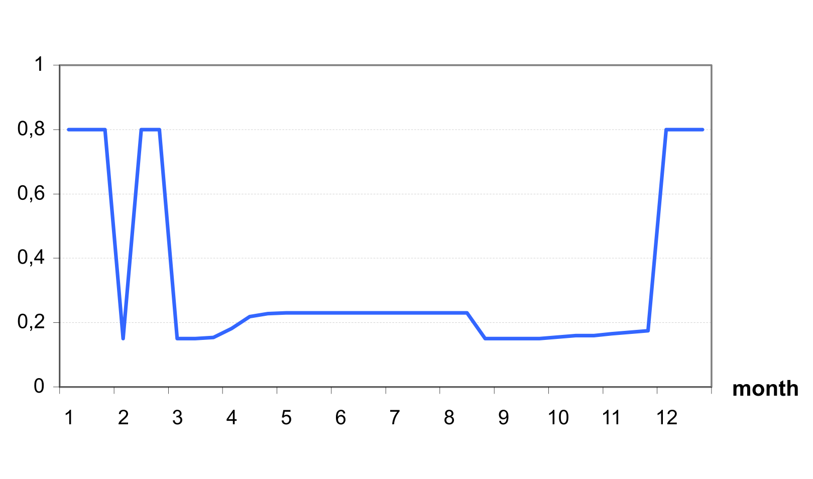
If a snow cover exists with 5 mm or greater water content, the value of albedo is set to 0.8. If the snow cover is less than 5 mm and no crop is growing, the soil albedo is set to the input value (default value = 0.15). An example on shows possible seasonal dynamics of albedo in a temperate zone with a maximum 0.8 in winter (snow cover), minimum in march and september (equal to the bare soil albedo), and increasing up to 0.23 in summer (crop growth).
2.1.7 Soil Evaporation and Plant Transpiration
The model calculates evaporation from soils and transpiration by plants separately using an approach similar to that of . The plant transpiration is calculated as \[\label{eq:60} \begin{array}{ll} EP=\frac{EO*LAI}{3}, & \quad 0\leq LAI \leq 3.0 \\ EP=EO, & \quad LAI>3.0 \end{array}\]
where EO is the potential evapotranspiration in mm d-1 estimated by , EP is the plant water transpiration rate in mm d-1 and LAI is the leaf area index (area of plant leaves relative to the soil surface area).
If soil water is limited, plant water transpiration is reduced. The approach is described in about water stress.
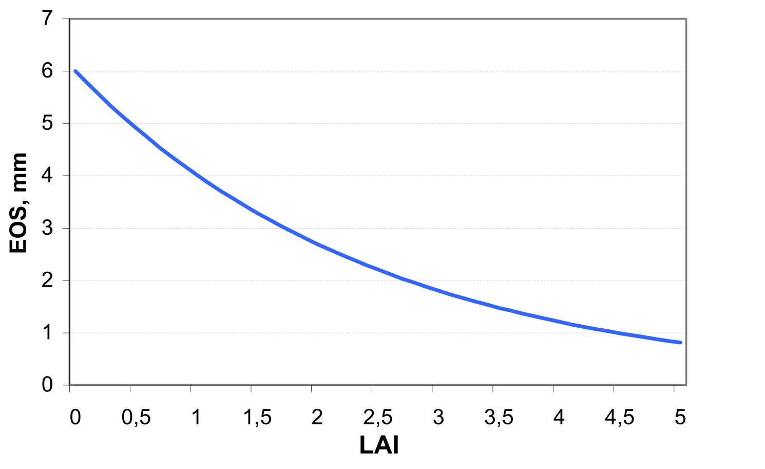
Potential soil evaporation ESO in mm d-1 is simulated by an exponential function of leaf area index LAI according to the equation of (see also ): \[\label{eq:61} ESO=EO*exp(-0.4*LAI)\]
Actual soil evaporation is calculated in two stages. In the first stage, soil evaporation is limited only by the energy available at the surface, and is equal to the potential soil evaporation. When the accumulated soil evaporation exceeds the first stage threshold (equal to 6 mm), the second stage begins. Then soil evaporation is estimated with the equation
\[\label{eq:62} ES=3.5*(\sqrt TST-\sqrt TST-1)\]
where ES is the soil evaporation for day t in mm d-1 and TST is the number of days since stage two evaporation began.
Actual soil water evaporation is estimated on the basis of the top 30 cm of soil and snow cover, if any. If the water content of the snow cover is greater or equal to ES, the soil evaporation comes from the snow cover. If ES exceeds the water content of the snow cover, water is removed from the upper soil layers if available.
2.1.8 Groundwater Flow
The groundwater submodel in the integrated river basin model like SWIM is intended for general use in regions where extensive field measurements are not available. Thus, the groundwater component has to be parameterized using readily available inputs. Also, it must have the level of sophistication similar to those of the other components. Therefore a detailed numerical model is not justified for this case, and a relatively simple yet realistic approach was chosen for use in SWAT and SWIM.
The simulated hydrological system consists of four control volumes that include:
the soil surface,
the soil profile or root zone,
the shallow aquifer, and
the deep aquifer.
The percolation from the soil profile is assumed to recharge the shallow aquifer. The surface runoff, the lateral subsurface flow from the soil profile, and return flow from the shallow aquifer contribute to the stream flow. The water balance equation for the shallow aquifer is \[\label{eq:63} SAW(t+1)=SAW(t)+RCH-REVAP-GWQ-SEEP\]
where SAW(t) is the shallow aquifer storage in the day t, RCH is the recharge, REVAP is the water flow from the shallow aquifer back to the soil profile, GWQ is the return flow or groundwater contribution to streamflow, SEEP is the percolation or seepage to the deep aquifer (all – in mm d-1), and t is the day.
REVAP is defined as water that raises from the shallow aquifer to the soil profile and is lost to the atmosphere by soil evaporation or plant root uptake.
The approach of , who derived the non-steady-state response of groundwater flow to periodic recharge from steady-state formula, is used \[\label{eq:64} GWQ=8*\frac{KD*GWH}{DS\textsuperscript{2}}\]
where KD is the hydraulic conductivity of groundwater in mm d-1, DS is the drain spacing in m, and GWH is the water table height in m.
Assuming that the shallow aquifer is recharged by seepage from stream channels, reservoirs, or the soil profile (rainfall and irrigation), and is depleted by the return flow to the stream, fluctuations of water table can be estimated using the equation of
\[\label{eq:65} \frac{d(GWH)}{dt} = \frac{RCH-GWQ}{0.8*SY}\]
where SY is the specific yield.
The return flow can be estimated assuming that its variation with time is also linearly related to the rate of change of the water table height: \[\label{eq:66} \frac{d(GWQ)}{dt}=10*\frac{KD*(RCH-GWQ)}{SY*DS\textsuperscript{2}}=RF*(RCH-GWQ)\]
where RF is the constant of proportionality or the reaction factor for groundwater.
Integration of gives \[\label{eq:67} GWQ(t+1)=GWQ(t)*exp(-RF*\Delta t)+RCH*\biggl[1-exp(-RF*\Delta t)\biggl]\]
The relationship for the water table height is derived combining and . It results in the following relationship \[\label{eq:68} GWH(t+1)=GWH(t)*exp(-RF*\Delta t)+\frac{RCH}{0.8*SY*RF}*\biggl(1.-exp(-RF*\Delta t)\biggl)\]
The percolation from the soil profile is assumed to recharge the shallow aquifer. The delay time or drainage time of the aquifer is used to correct the recharge. used an exponential decay weighting function proposed by to estimate the delay time for return flow in their precipitation / groundwater response model \[\label{eq:69} RCH(t+1)=\biggl(1.-exp\bigl(-\frac{1}{DEL}\bigl)\biggl)*RCH(t+1)+exp\bigl(-\frac{1}{DEL}\bigl)*RCH(t)\]
where DEL is the delay time or drainage time of the aquifer in days . This equation will affect only the timing of the return flow and not the total volume. The is used in SWIM to correct the recharge.
The volume of water flow from the shallow aquifer back to the soil profile, REVAP, is estimated with the equations \[\label{eq:70} \begin{array}{ll} REVAP=CR*ET, & \qquad REVAP>RST \\ REVAP=0, & \qquad REVAP \leq RST \end{array}\]
where ET is the actual evapotranspiration occurring in the soil profile, CR is the revap coefficient, and RST is the revap storage in mm.
The amount of percolation or seepage from the shallow aquifer (recharge to the deep aquifer) is estimated as a linear function \[\label{eq:71} SEEP=CS*RCH\] where CS is the seepage coefficient.
2.1.9 Transmission Losses
Many watersheds, especially in semiarid areas, have alluvial channels that abstract large quantities of stream flow . The abstractions, or transmission losses, reduce runoff volumes because water is lost when the flood wave travels downstream.
A procedure for estimating transmission losses for ephemeral streams is described by Lane in the SCS Hydrology Handbook , chapter 19. The procedure is based on derived regression equations for estimation of transmission losses in the absence of observed inflow outflow data. It enables the user to estimate transmission losses for similar channels of arbitrary length and width using channel geometry parameters (width and depth) and Manning’s "n". This procedure is used in SWIM as well as in SWAT to estimate transmission losses.
The unit channel intercept and slope, and the decay factor are estimated with regression equations obtained from the analysis of observed data in different conditions: \[AR=-0.001831*CHK*DU\]
\[DEC=-1.09*ln\biggl(1.-\frac{0.2649*CHK*DU}{VOLQ\textsubscript{in}}\biggl)\]
\[BR=exp(-DEC)\]
where AR is the unit channel intercept in m3, CHK is the effective hydraulic conductivity of the channel alluvium in mm h-1 , DU is the duration of streamflow in h, DEC is the decay factor in m km-1, VOLQin is inflow volume of m3, and BR is the unit channel regression slope.
The inflow volume is assumed to be equal to the surface runoff from the sub-basin. The flow duration DU in h is estimated from
\[DU=\frac{Q*A}{1.8*PEAKQ}\]
where Q is the surface runoff volume in mm, A is the drainage area in ha, and PEAKQ is the peak flow rate in m3 s-1.
The regression parameters are estimated as \[AX=\bigl[AR*(1-BR)\bigl]*(1-BR*CHL)\]
\[BX=CHL*CHW*exp(-2.04*DEC)\]
\[TH\textsubscript{0}=-\frac{AX}{BX}\]
where AX is the regression intercept in m km-1, BX is the regression slope, CHW is average width of flow in m, CHL is length of channel in km, and TH0 is the threshold volume for a unit channel in m3.
Then the final equation for runoff volume after losses, VOLQtr, is \[\begin{array}{ll} VOLQ\textsubscript{tr}=-AX+BX*VOLQ\textsubscript{in} & \quad VOLQ\textsubscript{in}>TH\textsubscript{0} \\ VOLQ\textsubscript{tr}=0 & \quad VOLQ\textsubscript{in}<TH\textsubscript{0} \end{array}\]
The final equation for peak discharge after losses PEAKQtr, is \[\begin{array}{ll} PEAKQ\textsubscript{tr}=\frac{12.1*AX}{DU-(1-BX)*VOLQ\textsubscript{in}+BX*PEAKQ\textsubscript{in}}, & \quad VOLQ\textsubscript{in}>0 \end{array}\]
where PEAKQin is the initial peak runoff rate.
2.2 Crop / Vegetation Growth
2.2.1 Crop Growth
The crop model in SWIM and SWAT is a simplification of the EPIC crop model . The SWIM model uses
a concept of phenological crop development based on daily accumulated heat units,
Monteith’s approach (1977) for potential biomass,
water, temperature, and nutrients stress factors, and
harvest index for partitioning grain yield.
However, the more detailed EPIC root growth and nutrient cycling modules are not included.
A single model is used for simulating all the crops and natural vegetation considered (see in ). The model is capable of simulating crop growth for both annual and perennial plants. Annual crops grow from planting date to harvest date or until the accumulated heat units equal the potential heat units for the crop. Perennial crops maintain their root systems throughout the year, although the plant may become dormant after frost. Later the term ‘crop’ will be used instead of ‘crop or natural vegetation’.
Phenological development of the crop is based on accumulation of daily heat units. The value of heat units accumulated in the day t, HUNA, is calculated as \[\label{eq:81} \begin{array}{lr} HUNA(t)=\biggl(\frac{TMX+TMN}{2}\biggl)-TB, & \quad HUNA\leq 0 \end{array}\]
where TMX and TMN are the maximum and minimum temperature in \(\,^{\circ}\mathrm{C}\), and TB is the crop specific base temperature in \(\,^{\circ}\mathrm{C}\) assuming that no growth occurs at or below TB.
Then the heat unit index IHUN ranging from 0 at planting to 1 at physiological maturity is calculated as \[\label{eq:82} IHUN=\frac{\sum_{t} \ HUNA(t) }{PHUN}\] where PHUN is the value of potential heat units required for the maturity of the crop. The values of PHUN for different crops are provided in the crop database supplemented with the model.
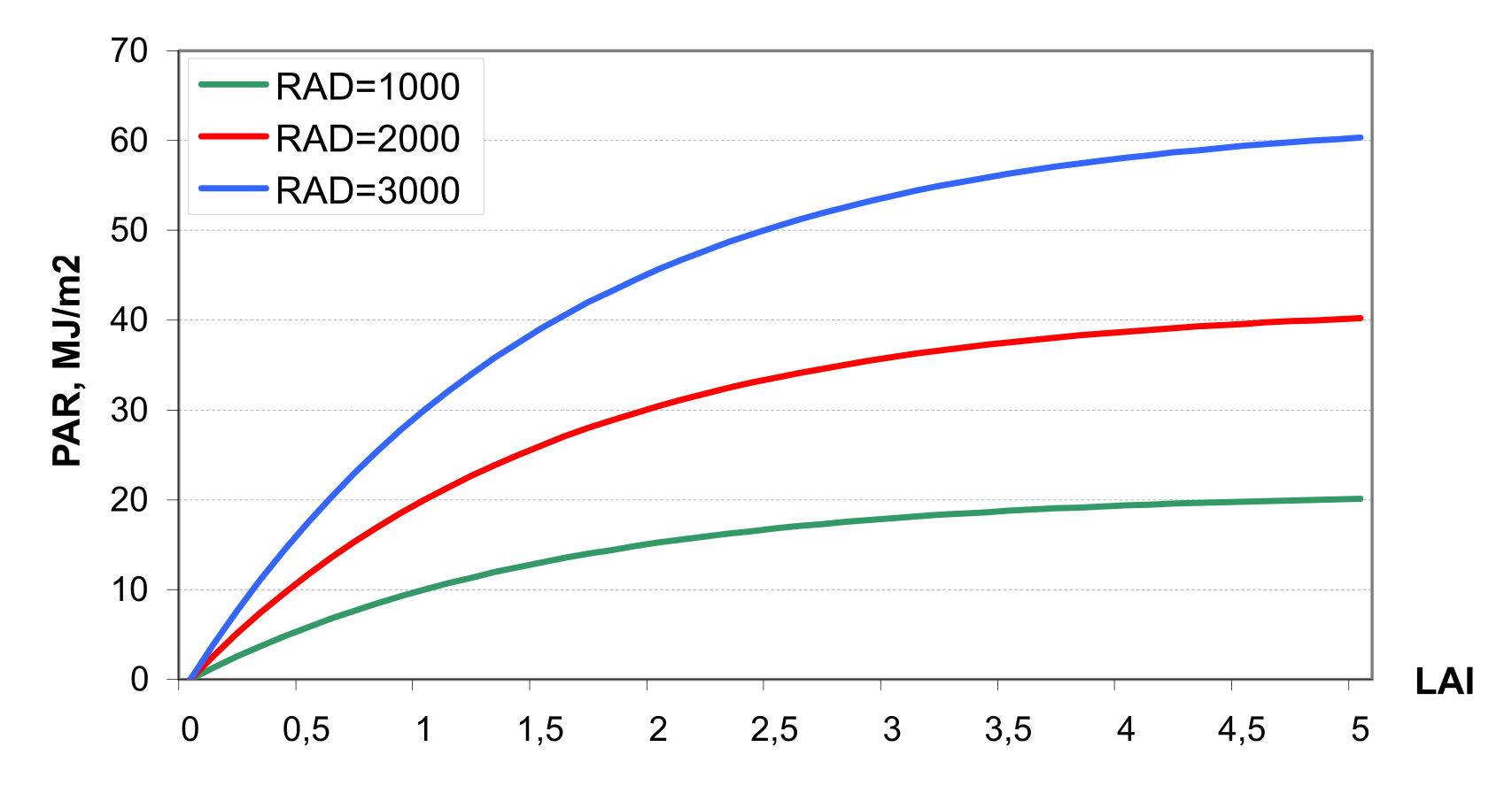
Interception of solar radiation is estimated with Beer’s law equation as a function of photosynthetic active radiation and leaf area index (see ) \[\label{eq:83} PAR=0.02092*RAD*\biggl[1-exp(-0.65*LAI)\biggl]\]
where PAR is the photosynthetic active radiation in MJ m-2, RAD is solar radiation in Ly, and LAI is the leaf area index.
Potential increase in biomass for a day is calculated using the approach of with the equation
\[\label{eq:84} \Delta BP=BE*PAR\]
where \(\Delta\)BP is the daily potential increase in total biomass in kg h-1 a-1, and BE is the crop-specific parameter for converting energy to biomass in kg m2 MJ-1 ha-1 d-1. The latter one is taken from the crop database.
The potential increase in biomass estimated with is adjusted daily if one of the plant stress factors is less than 1.0. The model considers stresses caused by water, nutrients, and temperature. The following equation is used to estimate the daily increase in biomass B (in kg ha-1) \[\label{eq:85} \Delta B= \Delta BP*REGF\]
where REGF is the crop growth regulating factor estimated as the minimum stress factor: \[\label{eq:86} REGF=min(WS,TS,NS,PS)\]
where WS, TS, NS, PS are stress factors caused by water, temperature, nitrogen and phosphorus, all varying between 0 and 1.
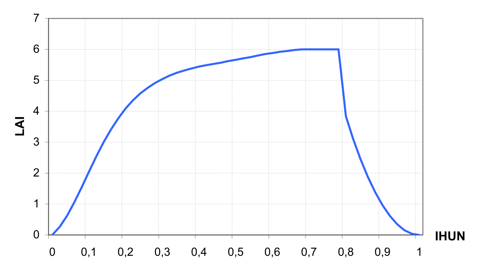
The leaf area index LAI is simulated as a function of heat units and biomass, differently for two phases of the growing season.
\[\label{eq:87} \begin{array}{ll} LAI=\frac{LAIMX*BAG}{BAG+exp(9.5-0.0006*BAG)}, & \quad IHUN\leq DLAI \\ LAI=16*LAIMX*(1-IHUN)\textsuperscript{2}, & \quad IHUN>DLAI \end{array}\]
where LAIMX is the maximum potential LAI for the specific crop, BAG is aboveground biomass in kg ha-1, and DLAI is the fraction of the growing season before LAI starts declining (crop-specific parameter). An example of LAI dynamics is shown in ).
The aboveground biomass is estimated as \[\label{eq:88} BAG=(1-RWT)*BT\] where RWT is the fraction of total biomass partitioned to the root system, and BT is total biomass in kg ha-1.
The fraction of total biomass partitioned to the root system normally decreases from 0.3 to 0.5 in the seedling to 0.05 to 0.20 at maturity . The model estimates the root fraction to range linearly from 0.4 at emergence to 0.2 at maturity using the equation \[\label{eq:89} RWT=(0.2-0.2*IHUN)\]
2.2.2 Growth Constraint: Water Stress
The water stress factor is calculated by considering water supply and water demand with the following equation \[\label{eq:90} WS=\frac{\sum_{i=1}^M WU\textsubscript{i}}{EP}\]
where WUi is plant water use in layer i in mm. The value of potential plant transpiration EP is calculated in the evapotranspiration module.
The plant water use is estimated using the approach of for simulating plant water uptake. First, the root depth is calculated with the equation \[\label{eq:91} RD=2.5*IHUN*RDMX\]
where RD is the fraction of the root zone that contains roots and RDMX is the maximum root depth in m (crop-specific parameter).
Then the potential water use in each soil layer is estimated with the equation \[\label{eq:92} WUP\textsubscript{i}=\frac{EP}{1-exp(RDP)}*\biggl(1-exp\bigl(-\frac{RDP*RZD\textsubscript{i}}{RD}\bigl)\biggl)\]
where WUPi is the potential water use rate from layer i in mm d-1, RDP is the rate depth parameter, and RZDi is the root zone depth parameter for the layer i in mm.
The latter one is defined as \[\label{eq:93} RZD\textsubscript{i}= \left\{ \begin{array}{rl} Z\textsubscript{i}, & RD>Z\textsubscript{i} \\ RD, & RD\leq Z\textsubscript{i} \end{array} \right\}\]
The value of RDP used in the model (3.065) was determined assuming that about 30% of the total water use comes from the top 10% of the root zone. The details of evaluating RDP are given in . allows roots to compensate for water deficits in certain layers by using more water in layers with adequate supply.
Then the potential water use must be adjusted for water deficits to obtain the actual water use WU for each layer: \[\label{eq:94} \begin{array}{ll} WU\textsubscript{i}=WUO\textsubscript{i}*\frac{SW\textsubscript{i}}{0.25*FC\textsubscript{i}}, & \quad SW\textsubscript{i}\leq 0.25*FC\textsubscript{i} \end{array}\]
\[\label{eq:95} \begin{array}{ll} WU\textsubscript{i}=WUP\textsubscript{i}, & \quad SW\textsubscript{i} > 0.25*FC\textsubscript{i} \end{array}\]
After the calculation of actual water use by plants, the plant transpiration EP is adjusted.
2.2.3 Growth Constraint: Temperature Stress
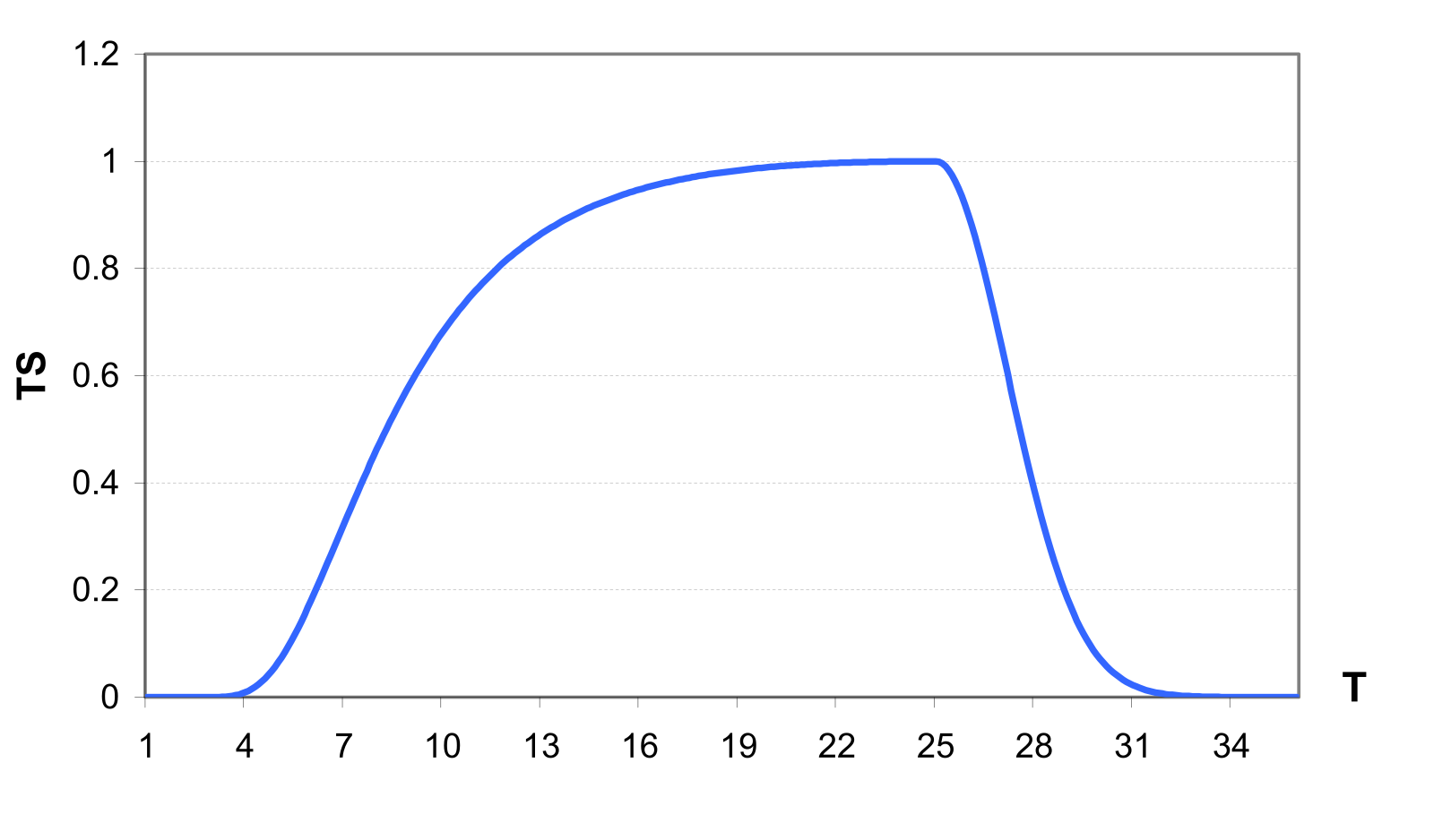
The temperature stress factor is calculated as an asymmetrical function, differently for temperature below the optimal temperature TO, and above it. The equation for the temperature stress factor TS for temperatures below TO is \[\label{eq:96} \begin{array}{rr} TS=exp\biggl(ln(0.9)*\bigl(\frac{CTSL*(TO-T)}{T+1.*10\textsuperscript{-6}}\bigl)\textsuperscript{2}\biggl), & T\leq TO \end{array}\]
where CTSL is the temperature stress parameter for temperatures below TO, and T is the daily average air temperature in °C. The temperature stress parameter CTSL is evaluated as \[\label{eq:97} CTSL=\frac{TO+TB}{TO-TB}\]
where TB is the base temperature for the crop in °C. assures that TS=0.9 when the air temperature is (TO+TB)/2.
For the temperatures higher than TO \[\label{eq:98} \begin{array}{rr} TS=exp\biggl(ln(0.9)*\bigl(\frac{CTSL*(TO-T)}{T+1.*10\textsuperscript{-6}}\bigl)\textsuperscript{2}\biggl), & T > TO \end{array}\]
where the temperature stress parameter for temperatures higher than TO, CTSH, is evaluated as \[\label{eq:99} CTSH=2*TO-T-TB\]
An example of the temperature stress factor calculated with and is shown in .
2.2.4 Growth Constraints: Nutrient Stress
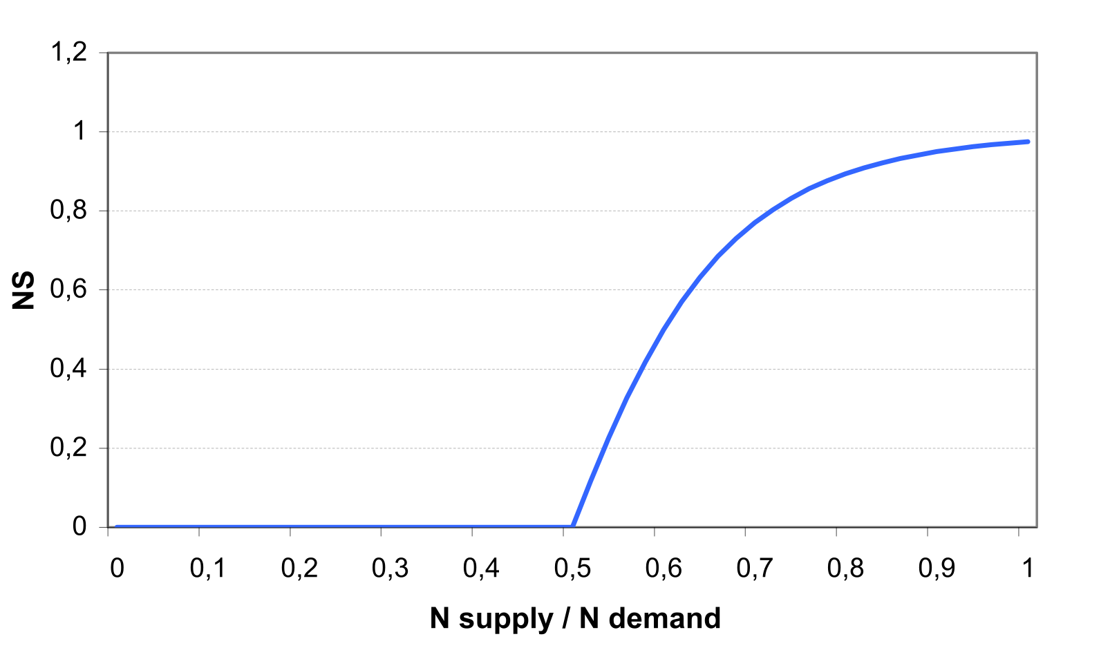
Estimation of nutrient stress factors is based on the ratio of simulated plant N and P contents to the optimal values of nutrient content. The stress factors vary non-linearly from 0 when N or P is half the optimal level to 1.0 at optimal N and P contents .
Let us consider the N stress factor first. As an initial step, the scaling factor SFN is calculated as \[\label{eq:100} SFN=200*\biggl(\frac{\sum UN(t)}{CNB*BT}-0.5\biggl)\]
where UN(t) is the crop N uptake on day t in kg ha-1, CNB is the optimal N concentration for the crop, BT is the accumulated total biomass in kg ha-1.
Then the N stress factor is calculated with the equation (see also ) \[\label{eq:101} \begin{array}{ll} NS=\frac{SFN}{SFN+exp(3.52-0.026*SFN)}, & \quad if SFN > 0 \end{array}\]
The P stress factor, PS, is calculated analogously, using the optimal P concentration, COP, instead.
2.2.5 Crop Yield and Residue
The economic yield of most crops is a reproductive organ. Harvest index (economic yield divided by aboveground biomass) is often a relatively stable value across a range of environmental conditions. Crop yield is estimated in the model using the harvest index concept \[YLD=HI*BAG\]
where YLD is the crop yield removed from the field in kg ha-1, HI is the harvest index at harvest, and BAG is the above ground biomass in kg ha-1.
Harvest index HIA increases non linearly during the growth season and can be estimated as the function of the accumulated heat units \[HIA=HVSTI*HIC\textsubscript{1}=HVSTI*\frac{100*IHUN}{100*IHUN+exp(11.1-10*IHUN)}\]
where HVSTI is the crop-specific harvest index under favourable growing conditions, and HIC1 is a factor depending on IHUN (see ).
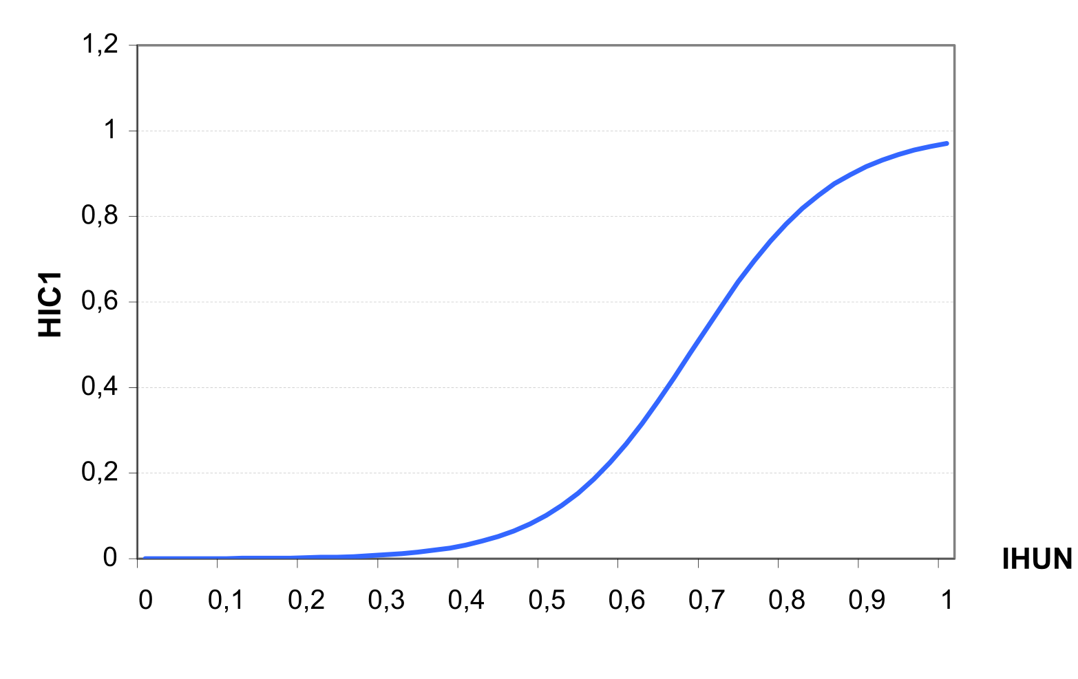
The constants in equation 103 are set to allow HIA to increase from 0.1 at IHUN=0.5 to 0.92 at IHUN=0.9. This is consistent with economic yield development of crops, which produce most economic yield in the second half of the growing season.
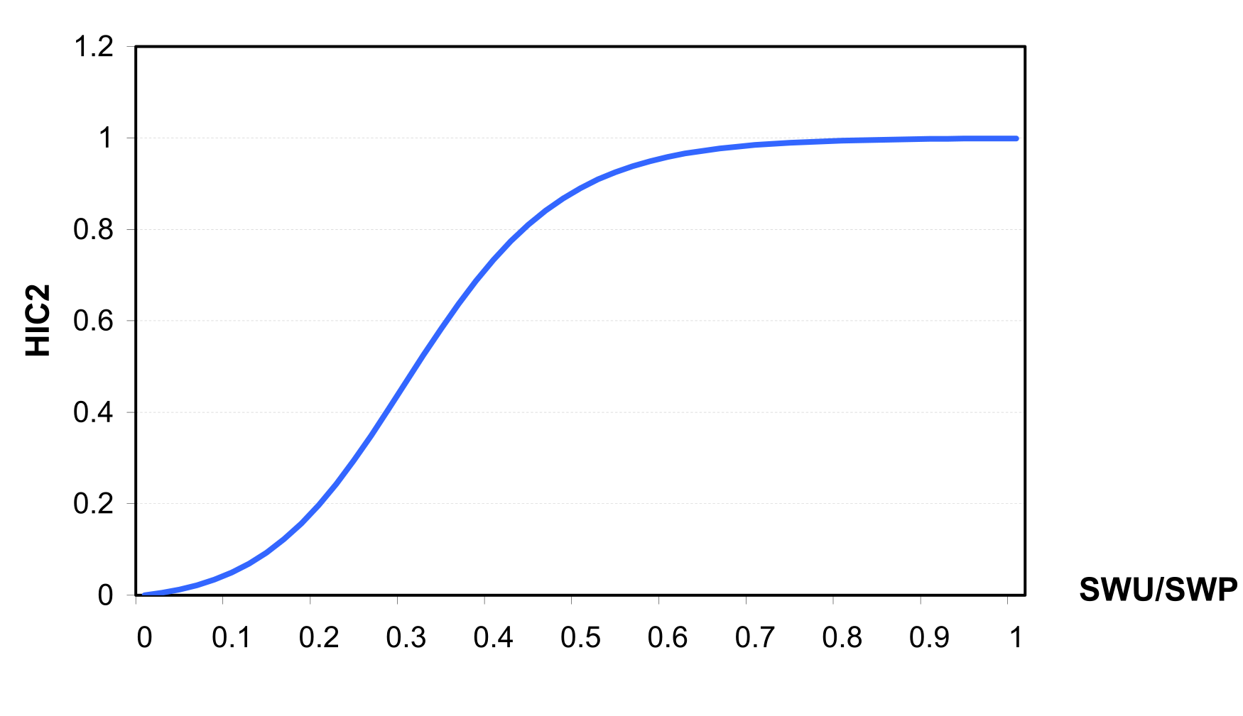
Most crops are particularly sensitive to water stress, especially in the second half of the growing season, when major yield components are determined . The effect of water stress on the harvest index is described by the following two equations \[HIAD=HIA*HIC\textsubscript{2}=HIA*\frac{WSF}{WSF+exp(6.117-0.086*WSF)}\]
\[WSF=100*\frac{SWU}{SWP+1.e\textsuperscript{-6}}\]
where HIAD is the adjusted harvest index, WSF is a parameter expressing water supply conditions for crop, HIC2 is a factor depending on WSF (see also factor HIC2 at ), SWU is accumulated actual plant transpiration in the second half of the growing season (IHUN>0.5), and SWP is accumulated potential plant transpiration in the second half of the growing season. The harvest index at harvest, HI is equal to HIAD.
The residue RSD is estimated at harvest as \[RSD=(1-RWT)*BT*HI\]
where RWT is the fraction of roots, and BT is the total biomass. This relationship can be modified for some crops if residue come from the roots.
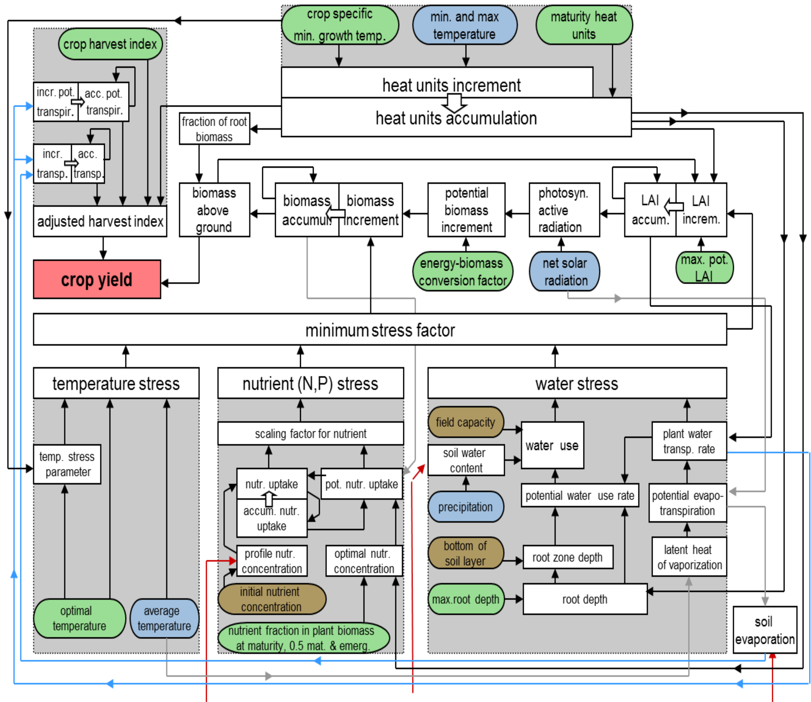
All processes described in – are presented graphically in . There are three basic blocks in the crop module (depicted by the grey coloured boxes) that are used to estimate the crop yield: accumulated heat units (top middle), stress factors (lower half), and harvest index (top left). The stress factors include temperature stress, nutrient stress (nitrogen and phosphorus), and water stress. The crop growth regulating factor is estimated as the minimum of these four factors. Nutrient stress is determined from the actual and potential nutrient uptake. Water stress is induced from water use and plant transpiration. The heat units accumulation is estimated from the crop specific minimum growth temperature, the daily minimum and maximum air temperatures and the assumed accumulated heat units. The adjusted harvest index is evaluated from the actual and potential transpiration and the crop specific harvest index. The small rectangles denote dependent variables, whereas the coloured ovals refer to model parameters independent from the others computed within the module. They describe the specifications of crop (green), climate (blue) and soil (brown).
2.2.6 Adjustment of Net Photosynthesis to Altered CO2
Different approaches for the adjustment of net photosynthesis and evapotranspiration to altered atmospheric CO2 concentration have been used in modelling studies . Detailed results about the interaction of higher CO2 and water use efficiency are described in .
Two different approaches can be used in SWIM for the adjustment of net photosynthesis (factor ALFA):
an empirical approach based on adjustment of the biomass-energy factor as suggested in EPIC and SWAT models , and
a new semi-mechanistic approach derived by F. Wechsung from a mechanistic model for leaf net assimilation , which takes into account the interaction between CO2 and temperature.
The second method and its application for climate change impact study with SWIM is described in
The factor ALFA is defined as \[\label{eq:107} ALFA=\frac{AS\textsubscript{2}}{AS\textsubscript{1}}\]
where AS1 and AS2 are net leaf assimilation rates (Mikro mol m-2 s-1) in two periods, corresponding to two different CO2 concentrations.
In the first method ALFA is estimated as \[\label{eq:108} ALFA=\frac{100*CA}{BE*\bigl(CA+exp(SHP\textsubscript{1}-CA*SHP\textsubscript{2})\bigl)}\]
where BE is the biomass-energy factor as in equation (83), CA is the current atmospheric CO2 concentration (micro mol mol-1), and SHP1 and SHP2 are the coefficients of the S-shape curve, describing the assumed change in BE for two different CO2 concentrations.
For the CO2 doubling, 1.1 times increase in BE is assumed for maize, and 1.3 times increase for wheat and barley (see ).
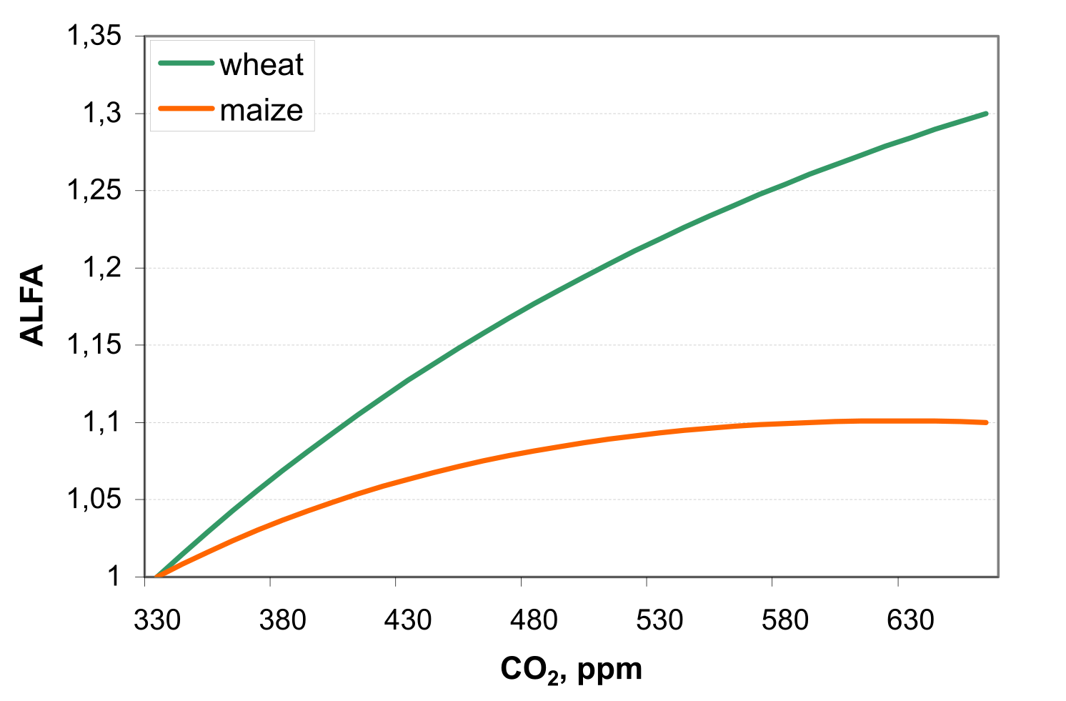
If CO2 concentration CA is changing from CA1 to CA2, and BE is changing from BE1 to BE2, the coefficients SHP1 and SHP2 can be estimated as following: \[\label{eq:109} SHP\textsubscript{2}=\frac{log(100*CA\textsubscript{1}/BE\textsubscript{1}-CA\textsubscript{1})-log(100*CA\textsubscript{2}/BE\textsubscript{2}-CA\textsubscript{2})}{CA\textsubscript{2}-CA\textsubscript{1}}\]
\[\label{eq:110} SHP\textsubscript{1}=log(100*CA\textsubscript{1}/BE\textsubscript{1}-CA\textsubscript{1})+CA\textsubscript{1}*SHP\]
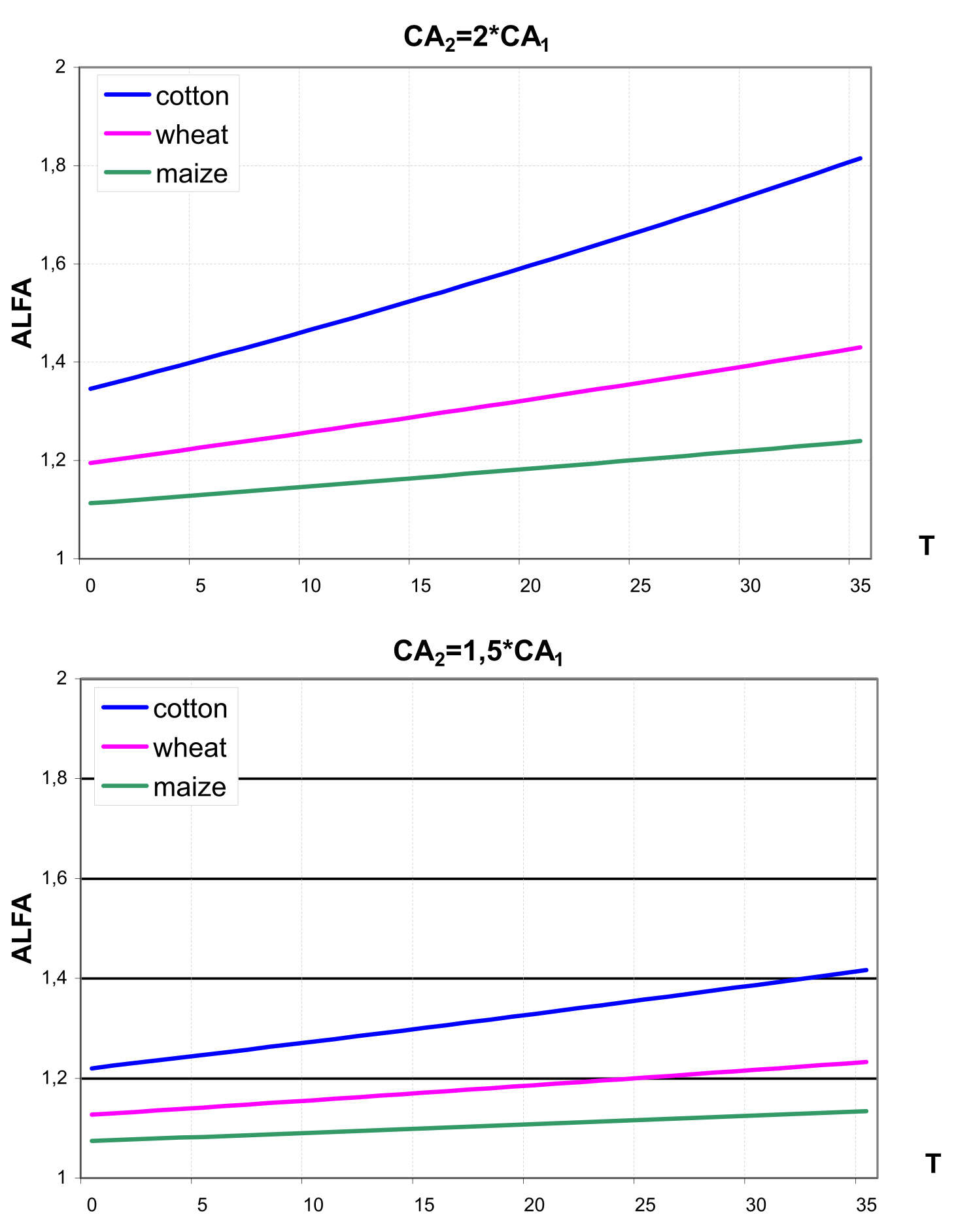
In the second method a temperature-dependent enhancement factor \(\alpha\) was derived from for cotton \[\label{eq:111} ALFA\textsubscript{COt}=exp\biggl[P\textsubscript{1}*(CL\textsubscript{2}-CL\textsubscript{1})-P\textsubscript{2}*\bigl((CL\textsubscript{2})\textsuperscript{2}-(CL\textsubscript{1})\textsuperscript{2}\bigl)+P\textsubscript{3}*TL*(CL\textsubscript{2}-CL\textsubscript{1})\biggl]\]
where TL is the leaf temperature (°C), CL1 and CL2 are the current and future CO2 concentration inside leaves (Mikro mol mol-1), and coefficients P1 = 0.3898*10-2 , P2 = 0.3769*10-5, and P3 = 0.3697*10-4.
It is assumed in the model that the leaf temperature TL coincides with the air temperature TX, and that the CO2 concentration inside leaves is a linear function of the atmospheric CO2 concentration: \[\label{eq:112} CL=0.7*CA\]
Then the cotton-specific factor ALFA was adjusted for wheat, barley and maize according to the latest crop-specific results reported in the literature \[\label{eq:113} ALFA\textsubscript{wheat}=(ALFA\textsubscript{cot})\textsuperscript{0.6}\] \[\label{eq:114} ALFA\textsubscript{barley}=(ALFA\textsubscript{cot})\textsuperscript{0.6}\] \[\label{eq:115} ALFA\textsubscript{maize}=(ALFA\textsubscript{cot})\textsuperscript{0.36}\]
which imply an increase in leaf net photosynthesis of 31, 31 and 10% for wheat, barley and maize, respectively, if the atmospheric CO2 increases from 360 to 720 ppm at 20°C and corresponds to the analogous assumption made in the first method. shows the temperature-dependent ALFA factor for cotton, wheat and maize in the case of CO2 doubling (a) and in the case of 50% increase in CO2 (b) assuming CA1 = 330 ppm estimated with the second method (,, , ).
2.2.7 Adjustment of Evapotranspiration to Altered CO2
Additionally, a possible reduction of potential leaf transpiration due to higher CO2 (factor BETA) derived directly from the enhancement of photosynthesis (factor ALFA) was taken into account in combination with both methods for the adjustment of net photosynthesis. The method was suggested by F. Wechsung.
The factor BETA is defined as \[\label{eq:116} BETA=\frac{EPO\textsubscript{2}}{EPO\textsubscript{1}}\] where EPO1 and EPO2 are potential plant transpiration rates (mol m-2 s-1) in two periods, corresponding to two different CO2 concentrations.
Assuming that \[\label{eq:117} \frac{AS}{EPO}=\frac{CA-CL}{VPD}*\frac{RESW}{RESC}\] where VPD is the vapour pressure deficit (kPa), RESC is the total leaf resistance to CO2 transfer (m2 s mol-1), RESW is the total leaf resistance to water vapour transfer (m2 s mol-1).
From definitions and and the ratio can be estimated \[\label{eq:118} \frac{ALFA}{BETA}=\frac{CA\textsubscript{2}-CL\textsubscript{2}}{CA\textsubscript{1}-CL\textsubscript{1}}*\frac{VPD\textsubscript{1}}{VPD\textsubscript{2}}~\frac{RESW\textsubscript{2}}{RESC\textsubscript{2}}*\frac{RESC\textsubscript{1}}{RESW\textsubscript{1}}\]
The following assumptions can be accepted for a given plant (see, e.g. ) \[\label{eq:119} \frac{RESW\textsubscript{2}}{RESC\textsubscript{2}}\approx\frac{RESW\textsubscript{1}}{RESC\textsubscript{1}}\] and \[\label{eq:120} VPD\textsubscript{2}\approx VPD\textsubscript{1}\] Then the following estimation is derived for BETA from , , and \[\label{eq:121} BETA=ALFA*\frac{CA\textsubscript{1}}{CA\textsubscript{2}}\]
postulate that on the regional scale there is no control of stomatal resistance on evapotranspiration, because the humidity profiles are adjusted within the planetary boundary layer. This response would counter stomatal closure as a negative feedback. On the other hand, recent model studies suggest that stomata have far more control on regional and global evapotranspiration than postulated by Jarvis and McNaughton .
Simulation runs with SWIM, which included the CO2 fertilization effect on crops, have been carried out applying both methods for ALFA factor in two variants: without and with factor BETA. In this way it is possible to account for current uncertainty regarding significance of stomatal effects on higher CO2 for regional evapotranspiration. The comparison of two methods for estimation of ALFA factor is shown in .
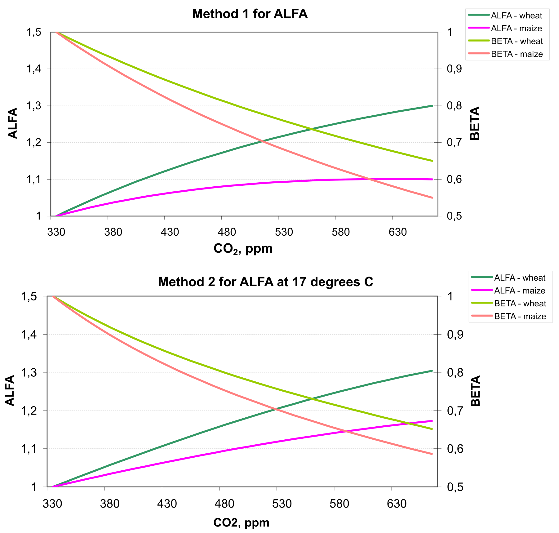
2.3 Nutrient Dynamics
Sub-basin nutrient cycling modules were taken from MATSALU and SWAT, and modified where necessary. The approach used in SWAT was modified from the EPIC model . The model simulates water, sediment and nutrients dynamics in every hydrotope, aggregates results for sub-basins, and then routes the water, sediment, and nutrients with lateral flow from the sub-basin outlet to the basin outlet.
2.3.1 Soil Temperature
Several processes of nutrient transformation, like mineralisation, are of microbial character, therefore estimation of soil temperature is necessary. Daily average soil temperature is defined at the center of each soil layer. The basic soil temperature equation is \[\label{eq:122} TSO(Z,t)=TAV+\frac{AMP}{2}*cos\biggl(\frac{2*\pi}{265}*(t-200)-\frac{Z}{DD}\biggl)*exp\biggl(-\frac{Z}{DD}\biggl)\]
where TSO(Z,t) is the soil temperature at the depth Z in the day t in °C, Z is depth from the soil surface in mm, t is time d, TAV is the average annual air temperature in °C, AMP is the annual amplitude in daily average temperature in °C, and DD is the damping depth for the soil in mm. The damping depth DD can be defined as a function of soil bulk density BD and water content SW as expressed in the following equations \[\label{eq:123} DD=DP*exp\biggl[ln(\frac{500}{DP})*\biggl(\frac{1-SPD}{1+SPD}\biggl)\textsuperscript{2}\biggl]\] \[\label{eq:124} DP=1000+\frac{2500*BD}{BD+686*exp(-5.63*BD)}\] \[\label{eq:125} SPD=\frac{SW}{(0.356-0.144*BD)*ZM}\]
where DP is the maximum damping depth for the soil in mm, BD is the soil bulk density in t m-3, ZM is the distance from the bottom of the lowest soil layer to the surface in mm, and SPD is a scaling parameter.
reflects average conditions, if only TAV and AMP parameters are used. Since air temperature is provided as input, the soil temperature module can use the air temperature as driver to correct .
First, the bare soil surface temperature is estimated as \[\label{eq:126} \begin{array}{ll} TGB(t)=WFT*(TMX-T)+T, & \quad PRECIP=0 \end{array}\]
\[\label{eq:127} \begin{array}{ll} TGB(t)=WFT*(T-TMN)+TMN, & \quad PRECIP>0 \end{array}\]
where TGB(t) is the bare soil surface temperature in °C in the day t, TMX, T, and TMN are the maximum, average and minimum daily air temperature in °C, and WFT is a proportion of rainy days in a month.
uses the minimum air temperature as a base to estimate surface temperature on rainy days. Higher temperatures are estimated on dry days using . The value of WFT is determined by considering the number of rainy days in this month: \[\label{eq:128} WFT=\frac{NRD}{NDD}\]
where NDD is the number of days in a month, and NRD is the number of rainy days in a month.
The soil surface temperature is also affected by residue and snow cover. This effect is introduced by lagging the predicted base surface temperature with the equation
\[\label{eq:129} TG(t)=BCV*TGB(t+1)+(1-BCV)*TGB(t)\]
where BCV is a lagging factor for simulating residue and snow cover effects on surface temperature. The value of BCV is 0 for bare soil and approaches 1.0 as cover increased as expressed in the equation \[\label{eq:130} BCV=max \left\{ \begin{array}{ll} \frac{COV}{COV+exp(7.563-1.297*10-4*COV)}, \\ \frac{SNO}{SNO+exp(6.055-0.3022*SNO)} \end{array} \right\}\]
where COV is the land cover, or the sum of above ground biomass and crop residue in kg ha-1 and SNO is the water content of the snow cover in mm.
Then the soil temperature at any depth is estimated with by substituting TG(t) for TS(0,t). TG(t) is a better estimate of the surface temperature than T(0,t), because current weather and cover conditions are considered. At the soil surface (Z=0), the proper substitution can be accomplished by adding TG(t) and subtracting TS(0,t) from . Differences between TG(t) and TS(0,t) are damped as Z increases. So, the final equation for estimating soil temperature at any depth is \[\label{eq:131} TSO(Z,t9)=TAV+\biggl(\frac{AMP}{2}*cos\biggl(\frac{2*pi}{365}*(t-200)-\frac{Z}{DD}\biggl)+TG(t)-TS(0,t)\biggl)*exp\biggl(-\frac{Z}{DD}\biggl)\]
An example of soil temperature dynamics as simulated by SWIM using equation 131 is shown in .
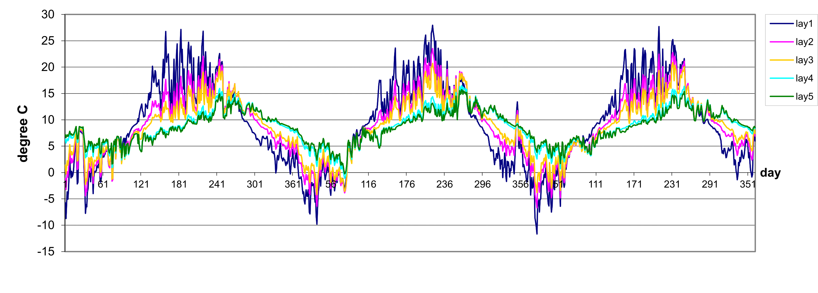
2.3.2 Fertilization and Input with Precipitation
Fertilization in form of mineral and active organic N and P is treated as input information in SWIM. The amounts and dates should be specified in advance. The amounts of fertilizers applied can be either strict or calculated values, depending on whether the strict or flexible fertilization scheme is applied. In the latter case the amounts of applied N and P depend on the actual concentration of mineral N and P in soil.
To estimate the N contribution from rainfall, SWIM uses an average rainfall N and P concentration, specific for the region. The amount of N and P in precipitation is estimated as the product of rainfall amount and concentration.
2.3.3 Nitrogen Mineralisation
The nitrogen mineralisation model is a modification of the PAPRAN mineralisation model . The model considers two sources of mineralisation:
fresh organic N pool, associated with crop residue, and
the active organic N pool, associated with the soil humus.
- Step 1.
When the model is initialized, organic N associated with humus is divided into two pools: active or readily mineralisable organic nitrogen ANOR and stable organic nitrogen SNOR (in kg ha-1) by using the equation \[\label{eq:132} ANOR=ANFR*NOR\]where ANFR is the active pool fraction (set to 0.15), NOR is the total organic N in kg ha-1 estimated from the initial soil data.
Organic N flow between the active and stable pools is described with the equilibrium equation \[\label{eq:133} ASNFL=CASN*\Biggl[\frac{ANOR}{ANFR}-SNOR\Biggl]\]
where ASNFL is the flow in kg ha-1 d-1 between the active and stable organic N pools, CASN is the rate constant (10-4 d-1). The daily flow of humus-related organic N, ASNFL, is added to the stable organic N pool and subtracted from the active organic N pool.
- Step 2.
The residue is decomposed daily in accordance with the equation \[\label{eq:134} RSD=RSD*(1-DECR)\]where DECR is the decomposition rate. Fresh organic N pool FON is associated with residue. It is recalculated with the same equation daily: \[\label{eq:135} FON=FON*(1-DECR)\]
and N mineralisation flow from fresh organic N in kg ha-1 d-1, FOMN, is estimated as \[\label{eq:136} FOMN=DECR*FON\]
The decomposition rate DECR is a function of C:N ratio, C:P ratio, temperature, and water content in soil \[\label{eq:137} DECR=0.05*min(CNRF, CPRF)*\sqrt{TFM\textsubscript{2}*WFM}\]
where CNRF and CPRF are the C:N and C:P ratio factors of mineralisation, respectively, and TFM2 and WFM are the temperature and soil water factors of mineralisation, respectively. The values of CNRF and CPRF are calculated with the equations \[\label{eq:138} CNRF=exp\biggl[-\frac{0.693*(CNR-25)}{25}\biggl]\] \[\label{eq:139} CPRF=exp\biggl[-\frac{0.693*(CPR-200)}{200}\biggl]\]
where CNR is the C:N ratio and CPR is the C:P ratio. The CNR and CPR are calculated with the equations \[\label{eq:140} CNR=\frac{0.58*RSD}{FON+NMIN}\] \[\label{eq:141} CPR=\frac{0.58*RSD}{FOP+PLAB}\]
where FON is the amount of fresh organic N in kg ha-1 , FOP is the amount of fresh organic P in kg ha-1, NMIN is the amount of mineral nitrogen (or nitrate nitrogen plus ammonium nitrogen) in kg ha-1, and PLAB is the amount of labile P in kg ha-1.
The temperature factor in is expressed by the equation (see also ) \[\label{eq:142} TFM\textsubscript{2}=\frac{TSO(2,t)}{TSO(2,t)+exp[6.82-0.232*TSO(2,t)]}\]
where TSO(2,t) is soil temperature in the second soil layer in °C (the depth of first layer is 10 mm). The soil water factor considers the relation of total soil water to field capacity \[\label{eq:143} WFM=\frac{SW}{FC}\]
The N mineralisation flow from residue, FOMN, calculated by is distributed between mineral nitrogen and active organic nitrogen pools in the proportion 4:1.
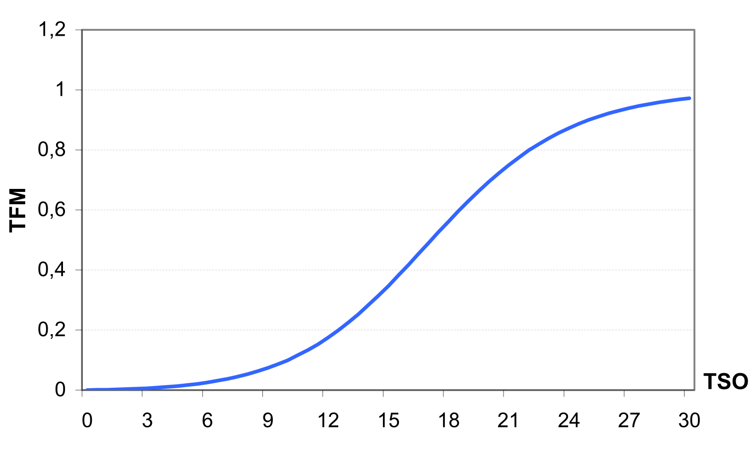
Temperature factor of mineralisation, TFM () - Step 3.
The stable organic N pool is not subjected to mineralisation. Only the active pool of organic N in soil is exposed to mineralisation. The mineralisation from the active organic N is expressed by the equation \[\label{eq:144} HUMN\textsubscript{i}=COMN*\sqrt{TFM\textsubscript{i}*WFM\textsubscript{i}}*ANOR\textsubscript{i}\] where HUMNi is the mineralisation rate in kg ha-1 d-1 for the active organic N pool in layer i, COMN is the humus rate constant for N (0.0003 d-1), and TFMi and WFMi are the temperature and water factors of mineralisation for the layer i.The temperature and water factors are calculated for any soil layer the same as for residue decomposition using and . At the end of the day, the humus mineralisation is subtracted from the active organic N pool and added to the mineral N pool.
2.3.4 Phosphorus Mineralisation
The phosphorus mineralisation model is structurally similar to the nitrogen mineralisation model, with some differences as explained below.
- Step 1.
Fresh organic P pool FOP is associated with residue. It is recalculated daily as \[FOP=FOP*(1-DECR)\]Then the P mineralisation flow from fresh organic P in kg ha-1 d-1, FOMP, is estimated as \[FOMP=DECR*FOP\]
where the rate DECR is calculated the same as for nitrogen using .
- Step 2.
Mineralisation of organic P associated with humus is estimated for each soil layer with the following equation \[HUMP\textsubscript{i}=COMP*\sqrt{TFM\textsubscript{i}*WFM\textsubscript{i}}*POR\textsubscript{i}\]where HUMPi is the mineralisation rate in kg ha-1 d-1 i, COMP is the humus mineralisation rate constant for P, and POR is the P organic pool in soil layer i.
To maintain the P balance at the end of a day, the mineralized humus is subtracted from the organic P pool and added to the mineral P pool, and the mineralized residue is subtracted from the FOP pool. Then 1/5 of FOMP is added to the POR pool, and 4/5 of FOMP is added to labile P pool, PLAB.
2.3.5 Phosphorus Sorption / Adsorption
Mineral phosphorus is distributed between three pools: labile phosphorus, PLAB, active mineral phosphorus, PMA and stabile mineral phosphorus, PMS. Mineral P flow between the active and stable mineral pools is governed by the equilibrium equation \[ASPFL=CASP*(4*PMA-PMS)\]
where ASPFL is the flow in kg ha-1 d-1 between the active and stable mineral P pools, CASP is the rate constant (0.0006 d-1). The daily flow ASPFL is added to the stable mineral pool and subtracted from the active mineral pool.
Mineral P flow between the active and labile mineral pools is governed by the equilibrium equation \[ALPFL=PLAB-CALP*PMA\]
where ALPFL is the flow in kg ha-1 d-1 between the active and labile mineral P pools, CALP is the equilibrium constant (default: 1.). The daily flow ALPFL is added to the active mineral pool and subtracted from the labile mineral pool.
2.3.6 Denitrification
Denitrification causes NO3 to be volatilized from soil. The denitrification occurs only in the conditions of oxygen deficit, which usually is associated with high water content. Besides, as one of the microbial processes, denitrification is a function of temperature and carbon content. The equation used to estimate the denitrification rate is \[\label{eq:150} \begin{array}{lr} DENIT\textsubscript{i}=WFD\textsubscript{i}*TCFD\textsubscript{i}*NIT\textsubscript{i}, & SW\textsubscript{i}/FC\textsubscript{i}\leq 0.9 \\ DENIT\textsubscript{i}=0. & SW\textsubscript{i}/FC\textsubscript{i}<0.9 \end{array}\]
where DENIT is the denitrification flow in layer i in kg ha-1 d-1, WFD is the soil water factor of denitrification, and TCFD is the combined temperature-carbon factor.
The soil water factor considers total soil water and is represented by the exponential equation (see ) \[\label{eq:151} WFD\textsubscript{i}=0.06*exp\biggl(\frac{3*SW\textsubscript{i}}{FC}\biggl)\]
where SWi is the soil water content in layer i in mm and FCi is the field capacity in mm mm-1.
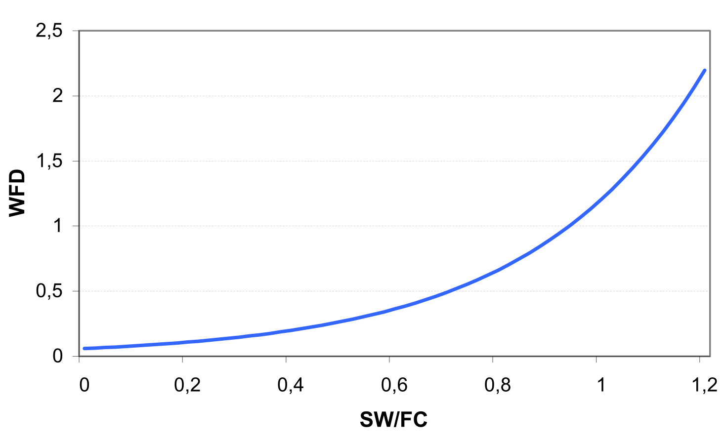
The combined temperature and carbon factor is expressed by the equation \[\label{eq:152} TCFD\textsubscript{i}=1-exp(CDN*TFM\textsubscript{i}*CBN\textsubscript{i})\]
where CDN is a shape coefficient, TFMi coincides with the temperature factor of mineralisation, and CBNi is the carbon content, and subscript i refers to the layers.
2.3.7 Nutrient Uptake by Crops
Nitrogen uptake by crop is estimated using a supply and demand approach. The daily (day t) crop N demand can be computed using the equation \[NDEM(t)=CNB(t)*BT(t)-CNB(t-1)*BT(t-1)\]
where NDEM(t) is the N demand of the crop in kg ha-1, CNB(t) is the optimal N concentration in the crop biomass, and BT(t) is the accumulated biomass in kg ha-1. Three parameters BN1, BN2, and BN3 are specified for every crop in the crop database, which describe: BN1 - normal fraction of nitrogen in plant biomass excluding seed at emergence, BN2 – at 0.5 maturity, and BN3 - at maturity.
Then the optimal crop N concentration is calculated as a function of growth stage using the equation (see also ) \[CNB=(BN\textsubscript{1}-BN\textsubscript{3})*\biggl[1-\frac{IHUN}{IHUN+exp(SP\textsubscript{1}-SP\textsubscript{2}*IHUN)}\biggl]+BN\textsubscript{3}\]
where SP1 and SP2 are shape parameters assuring the definition above, and IHUN(t) is the heat unit index expressing the fraction of the growing season as calculated in . The crop is allowed to take nitrogen from any soil layer that has roots. Uptake starts at the upper layer and proceeds downward until the daily demand is met or until all N has been depleted.
The same approach is used to estimate P uptake, differing only by the parameter values.
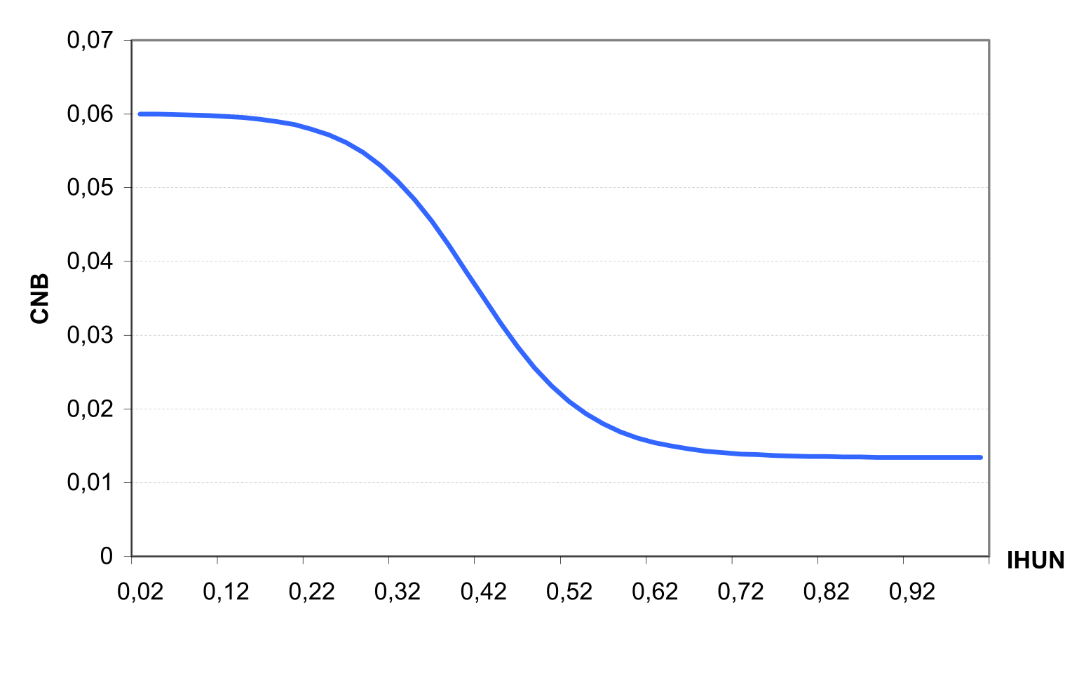
2.3.8 Nitrate Loss in Surface Runoff and Leaching to Groundwater
The total amount of water lost from the soil layer i is the sum of surface runoff, lateral subsurface flow (or interflow), and percolation from this layer: \[\label{eq:155} WTOT\textsubscript{i}=Q\textsubscript{i}+SSF\textsubscript{i}+PERC\textsubscript{i}\]
where WTOT is the total water lost from the soil layer in mm, Q is the surface runoff in mm, SSF is the lateral subsurface flow in mm, and PERC is the percolation in mm, and i is the layer.
The amount of nitrate nitrogen lost with WTOTi is the product of NO3-N concentration and water loss as expressed by the equation \[\label{eq:156} NFL\textsubscript{i}=WTOT\textsubscript{i}*CON\textsubscript{i}\] where NFLi is the amount NO3-N lost from the layer i in kg ha-1 and CONi is the concentration of NO3-N in the layer i in kg ha-1.
The amount of NO3-N left in the layer is adjusted daily as \[\label{eq:157} NMIN(t)=NMIN(t-1)-WTOT\textsubscript{i}*CON\textsubscript{i}\] where NMIN(t-1) and NMIN(t) are the amounts of NO3-N contained in the layer at the beginning and end of the day (in kg ha-1).
Then the NO3-N concentration can be estimated by dividing the weight of NO3-N by the water storage in the layer: \[\label{eq:158} CON\textsubscript{i}(t)=CON\textsubscript{i}(t-1)-CON\textsubscript{i}(t-1)*\biggl(-\frac{WTOT\textsubscript{i}}{PO\textsubscript{i}-WP\textsubscript{i}}\biggl)\]
where CONi(t) is the concentration of NO3-N at the end of the day in kg ha-1, PO is the soil porosity in mm mm-1, and WP is the wilting point water content for soil layer in mm mm-1.
is a finite different approximation of the exponential equation \[\label{eq:159} CON\textsubscript{i}(t)=CON\textsubscript{i}(t-1)-exp\biggl(-\frac{WTOT\textsubscript{i}}{PO\textsubscript{i}-WP\textsubscript{i}}\biggl)\]
Then the integration of allows to calculate NFL for any WTOT value \[\label{eq:160} NFL\textsubscript{i}=NMIN\textsubscript{i}*CW\textsubscript{i}=NMIN\textsubscript{i}*(1-exp(-\frac{WTOT}{PO\textsubscript{i}-WP\textsubscript{i}}))\]
The coefficient CW as the function of relative water content is depicted in . The average concentration for the day is \[\label{eq:161} CON\textsubscript{i}=\frac{NFL\textsubscript{i}}{WTOT\textsubscript{i}}\] Amounts of NO3-N contained in surface runoff, lateral subsurface flow, and percolation are estimated as the products of the volume of water and the concentration with .
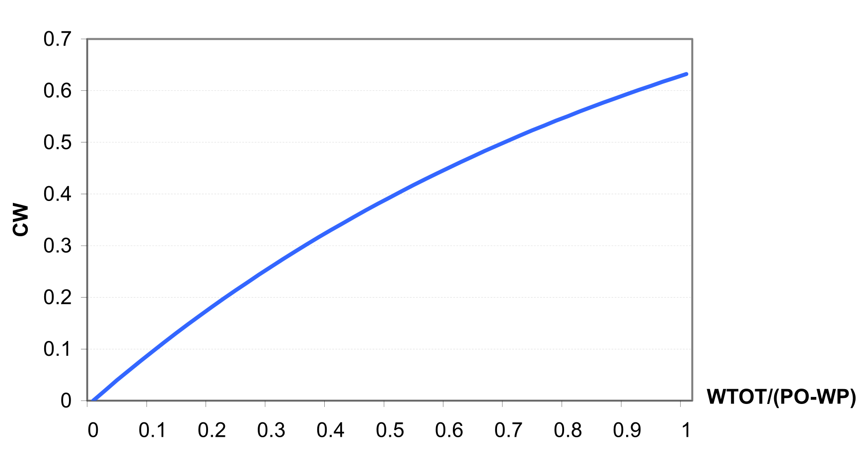
2.3.9 Soluble Phosphorus Loss in Surface Runoff
Phosphorus in soil is mostly associated with the sediment phase. Therefore the soluble P runoff equation can be expressed in the simple form \[PFL=\frac{0.01*COP*Q}{CSW}\]
where PFL is the soluble P in kg ha-1 d-1 lost with surface runoff, Q is the surface runoff in mm, COP is the concentration of labile phosphorus in soil layer in g t-1, and CSW is the P concentration in the sediment divided by that of the water in m3 t-1. The value of COP is input to the model and remains constant. The default value of CSW used in the model is 175.
All processes described in – are presented graphically in (for nitrogen cycle) and (for phosphorus).
The nitrogen module operates with four main pools depicted by the blue rectangles in : nitrate, stable organic N, mineralisable organic N and fresh organic N (crop residue). The nitrate pool is influenced by the following flows (depicted as flags): N fertilizer application, N precipitation input, N leaching, potential N uptake by plants and denitrification. The latter one is subject to the impact of the following variables and parameters: soil water content, field capacity, shape coefficient, temperature factor of mineralisation and carbon content. The exchange between stable and mineralisable organic nitrogen pools, whose intensity depends on the size of these pools and the rate constant, is shown on the right-hand side. The mineralisation is a function of soil temperature, soil water content, field capacity and the humus rate constant.
The phosphorus module () consists of five pools, namely fresh organic P (crop residue), organic P, labile P, active and stable mineral P. Labile P is influenced by the following five flows: decomposition, mineralisation, potential nutrient uptake, P loss by leaching and P exchange with the active mineral phosphorus pool. The size of the latter two flows is modulated by the amount of P in the concerned pools. The two-directional influence we meet in the case of the exchange flow between active and stable mineral P, and the mineralisation and decomposition flows (also pictured as flags). Mineralisation, decomposition, and soil erosion control the amount of organic P. The same as for the nitrogen cycle, mineralisation is influenced by soil temperature, soil water content, field capacity and the humus rate constant, whereas the decomposition rate essentially depends on the C-N-ratio, C-P-ratio and soil temperature.
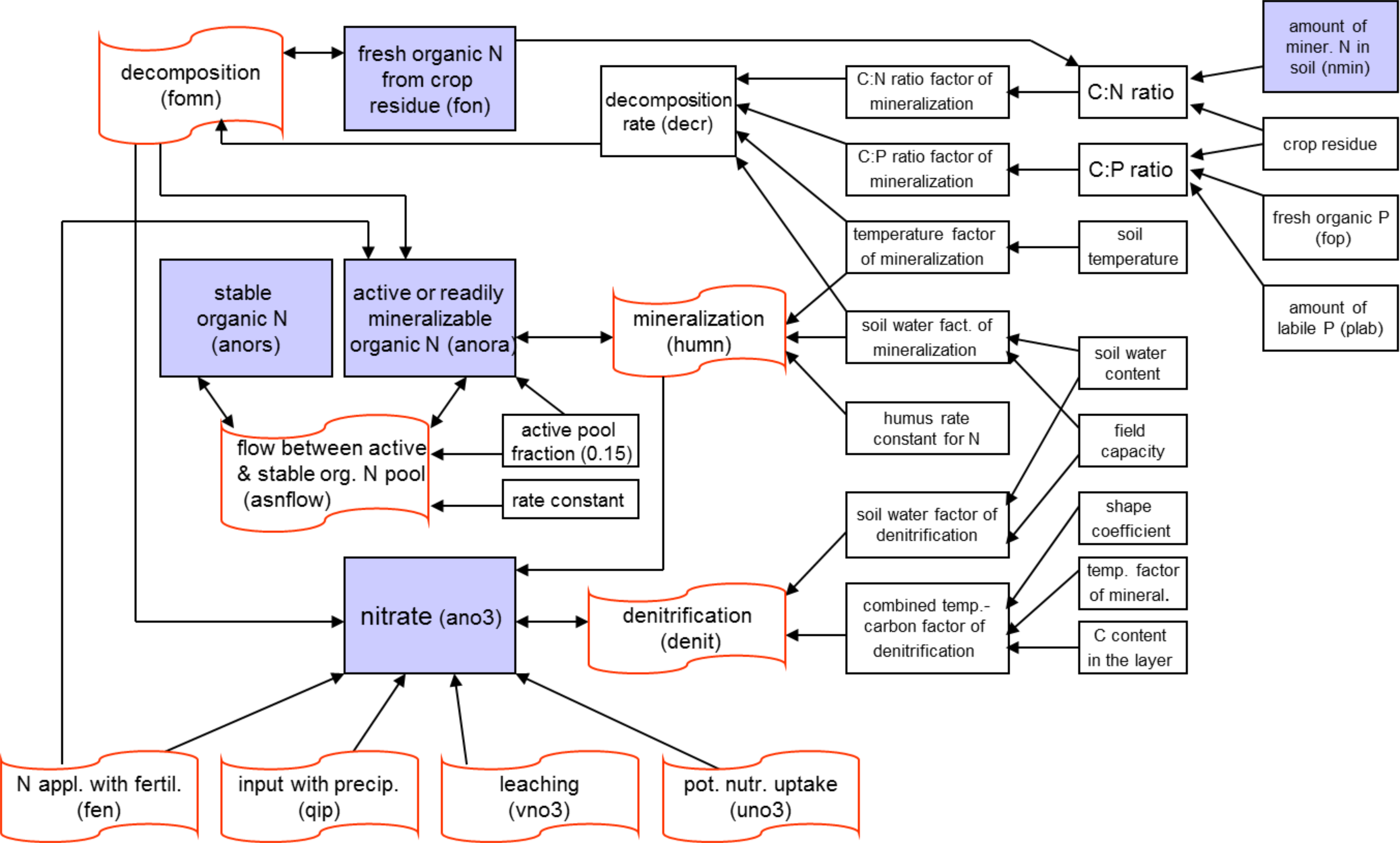
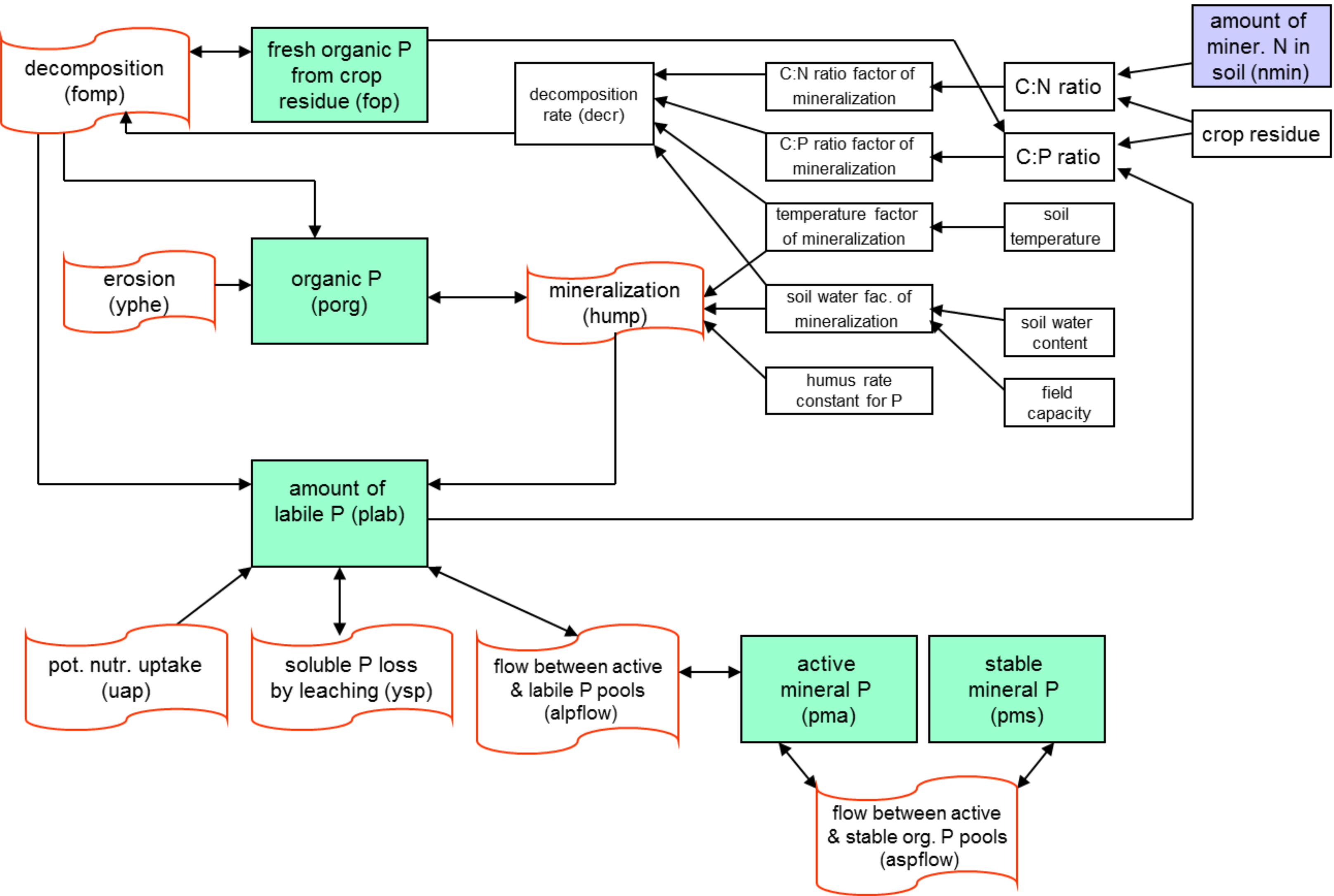
2.4 Erosion
2.4.1 Sediment Yield
Sediment yield is calculated for each sub-basin with the Modified Universal Soil Loss Equation (MUSLE) , practically the same as in SWAT: \[YSED=11.8*(VOLQ*PEAKQ)\textsuperscript{0.56}*K*C*ECP*LS\]
where YSED is the sediment yield from the sub-basin in t, VOLQ is the surface runoff column for the sub-basin in m3, PEAKQ is the peak flow rate for the sub-basin in m3 s-1, K is the soil erodibility factor, C is the crop management factor, ECP is the erosion control practice factor, and LS is the slope length and steepness factor.
The only difference between SWAT and SWIM in the erosion module is that the surface runoff, the soil erodibility factor K and the crop management factor C are estimated in SWIM for every hydrotope, and then averaged for the sub-basin (weighted areal average). In SWAT there are two options: option 1 based on two-level disaggregation “basin – sub-basins”, when the above mentioned factors are first estimated for the sub-basins, and option 2 similar to that of SWIM, when the factors are estimated first for HRUs (Hydrologic Response Units).
The soil erodibility factor K is estimated from the texture of the upper soil layer or is taken from a database.
The crop management factor, C, is evaluated with the equation, \[C=exp\bigl[CMN+(-0.2231-CMN)*exp(-0.00115*COV)\bigl]\] where COV is the soil cover (above ground biomass + residue) in kg ha-1 and CMN is the minimum value of C.
The value of CMN is estimated from the average annual value of C factor, CAV, using the equation \[CMN=1.463*ln(CAV)+0.1034\] The value of CAV for each crop is determined from tables prepared by .
The erosion control practice is estimated as default value of 0.5, if no other data are available (which is usually the case for mesoscale basins and regional case studies).
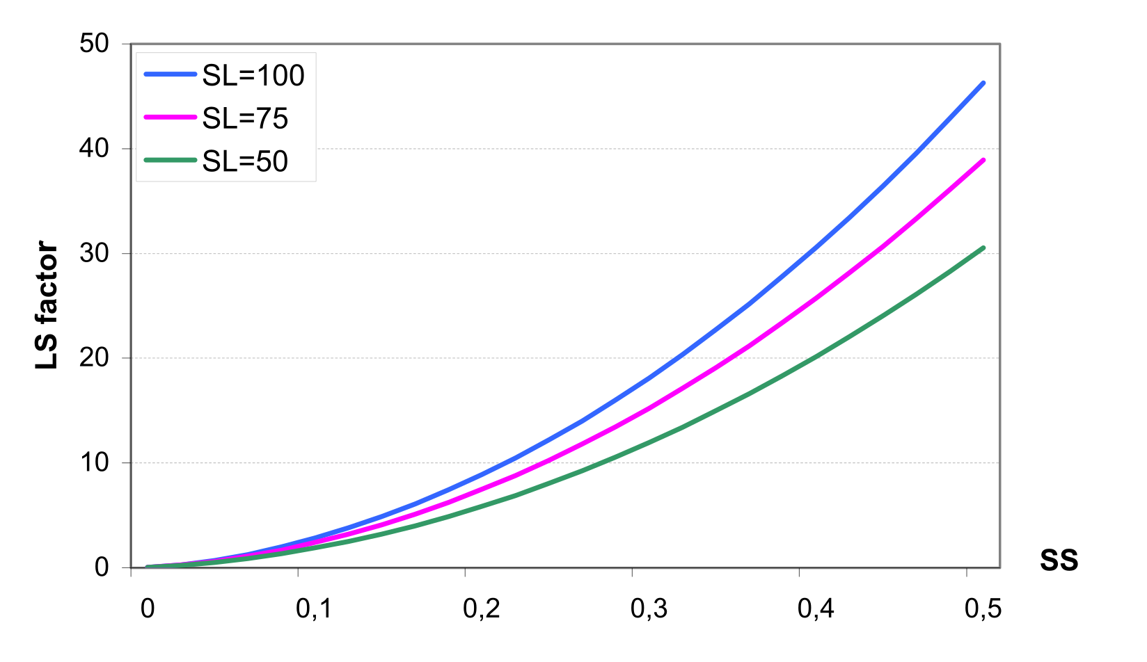
The LS factor is estimated with the equation (see ) \[\label{eq:166} LS=\biggl(\frac{SL}{22.1}\biggl)\xi*(65.41*SS2+4.565*SS+0.065)\] where SL is the slope length, SS is the slope steepness, and the exponent \(\xi\) varies with slope and is computed with the equation
\[\label{eq:167} \xi=0.6*\biggl[1-exp(-35.835*SS)\biggl]\] The slope length and slope steepness are calculated in SWIM/GRASS interface for every sub-basin.
2.4.2 Organic Nitrogen Transport by Sediment
A loading function developed by and modified by for application to individual runoff events is used to estimate organic N loss for each sub-basin. The loading function is \[\label{eq:168} YON=0.001*YSED*CNOR*ER\] where YON is the organic N runoff loss at the sub-basin outlet in kg ha-1, CNOR is the concentration of organic N in the top soil layer in g t-1, and ER is the enrichment ratio. The value of CNOR is input to the model and is constant throughout the simulation.
The enrichment ratio is the concentration of organic N in sediment divided by that of the soil. Enrichment ratios are logarithmically related to sediment concentration as described by . An individual event enrichment sediment concentration relationship was developed considering upper and lower bounds. The upper bound of the enrichment ratio is the inverse of the sediment delivery ratio DR (sub-basin sediment yield divided by gross sheet erosion): ER<1/DR. Exceeding the inverse of the delivery ratio implied that more organic N leaves the watershed than is dislodged from the soil.
The delivery ratio is estimated for each runoff event using the equation \[\label{eq:169} DR=\biggl(\frac{PEAKQ}{PRER}\biggl)\textsuperscript{0.56}\] where DR is the sediment delivery ratio, PEAKQ is the peak runoff rate in mm h-1, and PRER is the peak rainfall excess rate in mm h-1.
is based on sediment yield estimated using MUSLE . The rainfall excess rate cannot be evaluated directly because the model uses only the total daily runoff volume, and not the event rainfall. An estimation of PRER can be obtained, however, using the equation \[\label{eq:170} PRER=PRR-AIR\] where PRR is the peak rainfall rate in mm h-1 and AIR is the average infiltration rate in mm h-1.
The peak rainfall rate can be calculated with the equation \[\label{eq:171} PRR=2*PRECIP*log\biggl(\frac{1}{1-\alpha\textsubscript{0.5}}\biggl)\]
The average infiltration rate can be calculated with the equation \[\label{eq:172} AIR=\frac{PRECIP-Q}{DUR}\] where DUR is the rainfall duration in h, and PRECIP is rainfall in mm.
The rainfall duration is estimated the same as in according to . \[\label{eq:173} DUR=\frac{4.605*PRECIP}{PRR}=-\frac{2.3025}{log(1-\alpha\textsubscript{0.5})}\]
The enrichment ratio is estimated with the logarithmic equation \[\label{eq:174} ER=PCON*SEDC\textsuperscript{PEXP}\] where SEDC is the sediment concentration in g m-3, and PCON and PEXP are parameters set by the upper and lower limits.
To approach the lower limit for the enrichment ratio, 1.0, the sediment concentration should be extremely high. Conversely, a very low sediment concentration would cause the enrichment ratio to approach 1/DR. The simultaneous solution of at the boundaries assuming that sediment concentrations range from 500 to 250000 g m-3 gives the following estimations for PEXP and PCON \[\label{eq:175} PEXP=\frac{log(\frac{1}{DR})}{2.699}\] \[\label{eq:176} PCON=\frac{1}{0.25\textsuperscript{PEXP}}\]
2.4.3 Phosphorus Transport by Sediment
Phosphorus transport with sediments is simulated with a loading function similar to that described in for the organic N transport. The loading function for phosphorus is \[\label{eq:177} YP=0.01*YSED*POR\textsubscript{1}*ER\] where YP is the sediment phase of P loss in runoff in kg ha-1, and POR1 is the concentration of organic P in the top soil layer in g t-1.
2.5 River Routing
2.5.1 Flow Routing
The model uses the Muskingum flow routing method (see and ). For a given reach, the continuity equation may be expressed as: \[\label{eq:178} \frac{d(STOR)}{dt}=QIN(t)-QOUT(t)\]
where d(STOR)/dt is the rate of change of storage within the reach (m3 s-1), QIN(t) is the inflow rate (m3 s-1) at time t, and QOUT(t) is the outflow rate (m3 s-1) at time t. The Muskingum method assumes a variable discharge storage equation: \[\label{eq:179} STOR(t)=KST*\biggl[X*QIN(t)+(1-X)*QOUT(t)\biggl]\]
where STOR(t) is the storage (m3) in river reach at time t, KST is the storage time constant for the reach (s), and is the dimentionless weighting factor in river reach routing.
Here KST is the ratio of storage to discharge and has the dimention of time. In physical terms, KST is considered to be an average reach travel time for a flood wave, and X indicates the relative importance of the input QIN and outflow QOUT in determining the storage in a reach. The lower and upper limits for X are 0 and 0.5, respectively. Typical values of X for a river reach range between 0.0 and 0.3, with a mean value near 0.2.
Thus, from the change in storage over time \(\Delta\)t is given as \[\label{eq:180} \begin{array}{lr} STOR(t+1)-STOR(t)=KST*\biggl[X*QIN(t+1)+(1-X)*QOUT(t+1)\biggl] \\ -KST*\bigl[X*QIN(t)+(1-X)*QOUT(t)\bigl] \end{array}\]
The Muskingum equation is derived from the finite difference form of the continuity and as the following: \[\label{eq:181} QOUT(t+1)=C\textsubscript{1}*QIN(t+1)+C\textsubscript{2}*QIN(t)+C\textsubscript{3}*QOUT(t)\]
where the parameters C1, C2 and C3 are determined as (see also ) \[\label{eq:182} C\textsubscript{1}=\frac{-KST*X+0.5*\Delta t}{KST-KST*X+0.5*\Delta t}\] \[\label{eq:183} C\textsubscript{2}=\frac{KST*X+0.5*\Delta t}{KST-KST*X+0.5*\Delta t}\] \[\label{eq:184} C\textsubscript{3}=\frac{KST-KST*X-0.5*\Delta t}{KST-KST*X+0.5*\Delta t}\]
Here KST and \(\Delta\)t must have the same time units and the three coefficients C1, C2 and C3 sum to 1.0. Numerical stability is attained and the computation of negative outflows is avoided if the following condition is fulfilled \[\label{eq:185} 2*KST*X<\Delta t<2*KST*(1-X)\]
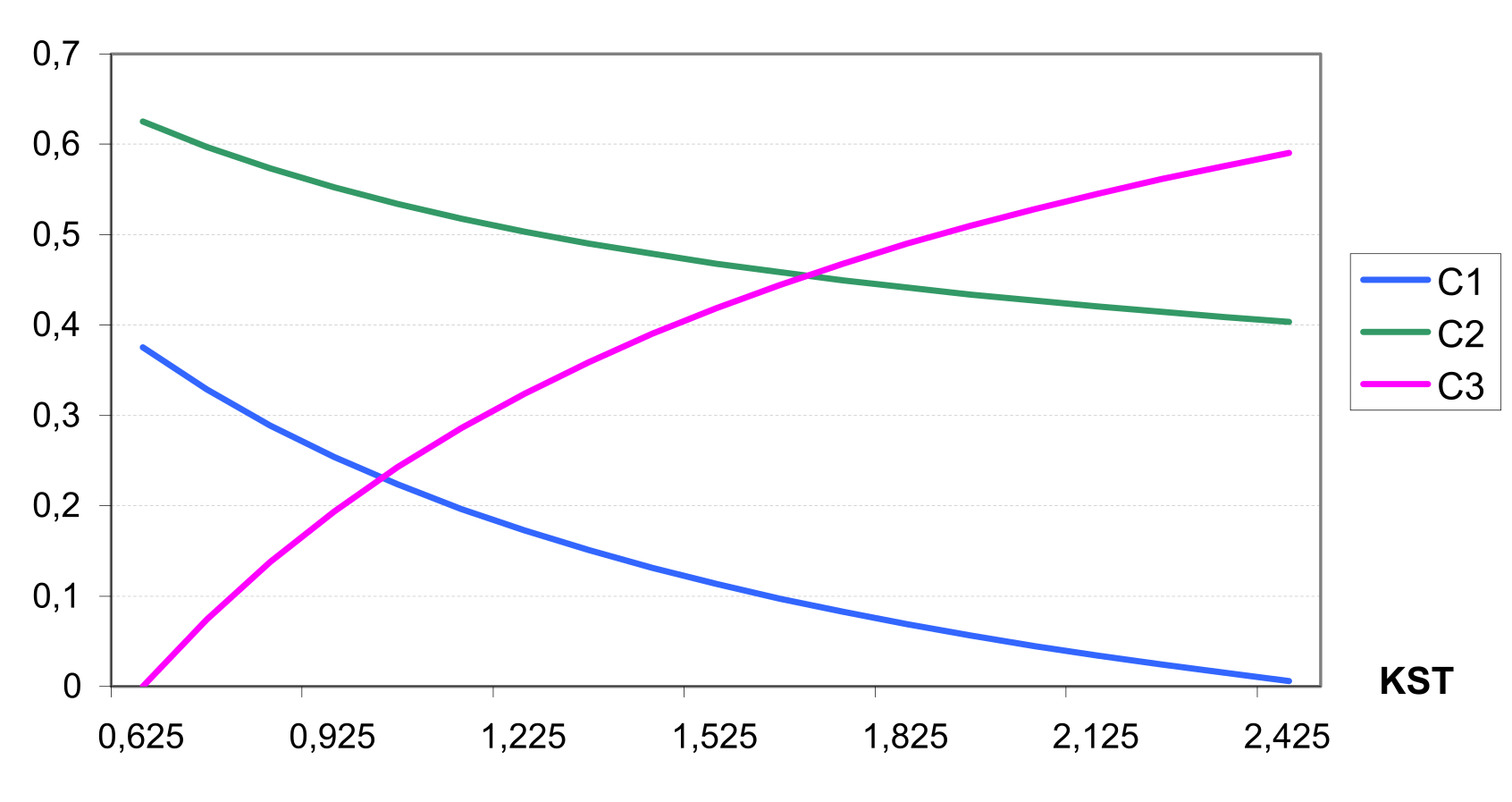
Fig. 2.26
Estimation of KST is based on the reach geometry \[\label{eq:186} KST=\frac{CHL}{CLR}\] where CHL is the reach length, and CLR is the wave celerity.
The celerity may be estimated by using the Manning formula with an adjusting coefficient for a certain reach shape. For the wide rectangular reach the celerity may be estimated (Schulze, p. AT13-9) as \[\label{eq:187} CLR=\frac{5*CHV}{3}\]
where CHV is the average stream velocity in m s-1. The average velocity is estimated from the Manning formula as \[\label{eq:188} CHV=\frac{HR\textsuperscript{2/3}*\sqrt{CHS}}{CHN}\]
where HR is hydraulic radius, CHS is channel bottom slope, CHN is the Manning’s roughness N. The value of X is set in the model to 0.2.
2.5.2 Sediment Routing
The sediment routing model consists of two components operating simultaneously – deposition and degradation in the streams. Deposition in the stream channel is based on the stream velocity in the channel, which is estimated as a function of the peak flow rate, the flow depth, and the average channel width with the equation \[CHV=\frac{PEAKQ}{FD*CHW}\] where CHV is the stream velocity in the channel in m s-1, PEAKQ is the peak flow rate in m3 s-1, FD is the flow depth in m, and CHW is the average channel width in m.
The flow depth is calculated using the Manning’s formula as \[FD=\biggl(\frac{PEAKQ*CHN}{CHW*\sqrt{CHS}}\biggl)\textsuperscript{0.6}\]
where CHN is the channel roughness, N, and CHS is the channel slope in m m-1.
The sediment delivery ratio DELR through the reach is described by the logarithmic equation suggested by J. Williams (similar to ) \[\label{eq:191} DELR=\frac{Q}{YSED\textsubscript{in}}*SPCON*CHV\textsuperscript{spexp}\]
where YSEDin is the sediment amount entering the reach, and the parameters SPCON (between 0.0001 and 0.01) and SPEXP (between 1.0 and 1.5) can be used for calibration. The power function in 191 is shown in for different combinations of SPCON and CHV.
If DELR < 1.0, the degradation is zero, and deposition is estimated from the sediment input as \[\label{eq:192} \begin{array}{lr} DEP=YSED\textsubscript{in}*(1-DELR), & DEGR=0 \end{array}\]
Otherwise, if DELR\(\leq\)1. the deposition is zero, and the degradation is calculated from the sediment input as \[\label{eq:193} \begin{array}{lr} DEP=0. \\ DEGR=YSEDin*(DELR-1)*CHK*CHC \end{array}\] where CHK is the channel K factor or the effective hydraulic conductivity of the channel alluvium (see also ), and CHC is the channel C factor.
Finally, the amount of sediment reaching the sub-basin outlet, YSEDout, is \[\label{eq:194} YSED\textsubscript{out}=YSED\textsubscript{in}-DEP+DEGR\]
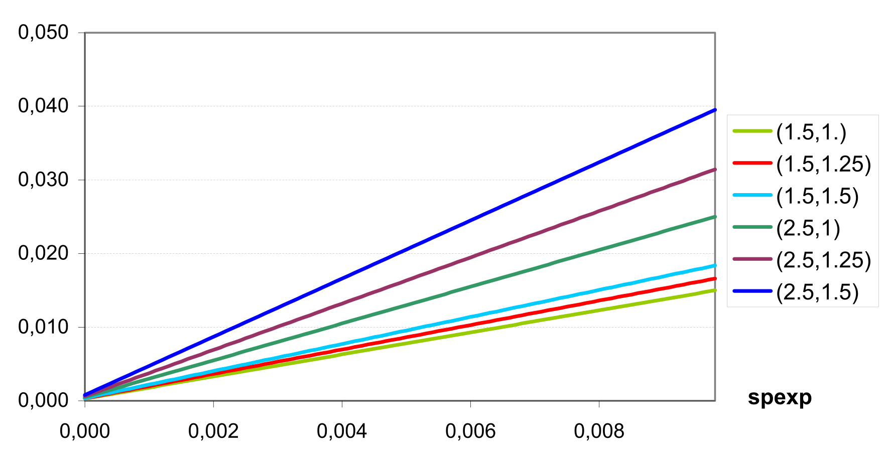
2.5.3 Nutrient Routing
Nitrate nitrogen and soluble phosphorus are considered in the model as conservative materials for the duration of an individual runoff event . Thus they are routed by adding contributions from all sub-basins to determine the basin load.
3 SWIM Code Structure and Input Parameters
In this chapter the code structure of the both parts of the modelling system:
the SWIM/GRASS interface, and
the simulation part of SWIM
are described. The SWIM/GRASS interface is applied to prepare necessary (but not all) input files to run the simulation part of SWIM. The simulation part of SWIM performs simulation of ecohydrological processes in river basins or regions.
In the code structure of the SWIM/GRASS interface is given, and in the code of the SWIM simulation part is described. The latter is described in more detail. The code development is continuing, and it is assumed that SWIM users should be able to understand and, if necessary, to modify some modules/subroutines of the simulation part or add new modules. Therefore the latter is described in more detail.
In input and output files are described, and in all input parameters are listed and defined.
3.1 Structure of the SWIM/GRASS Interface
It is recommended to read the overview of SWIM/GRASS interface () before reading this section.
The code includes menus and all menu-driven operations as described in . The subroutine main displays the first menu, which allows either to create a new project, or to copy, remove, or work on an existing project. The subroutine main_menu() provides the main menu, which lists steps to be completed by the interface.
When the step is chosen, the sub_menu() switches between the following important subroutines (see ):
get_basin_info - to request and extract a basin information from the user supplied map layer,
hydro_struct_swim – to create structure file for a basin based on basin map, land use map and soil map,
get_topo_info – to request an elevation map and extract the topographic properties using programs
ram.sub-basin and compute_slp_len,
rw_gw_swim – to read the extracted groundwater properties and write them in SWIM format,
com_rout_info_swim – to compute routing structure, including basin number, starting elevation, ending elevation, starting and ending accumulation cells, stream length and the next draining sub-basin number
get_climate_station_s – to extract the numbers of nearest 3 climate stations for a basin or each sub-basin,
get_precipit_station_s – to extract the number of nearest 3 precipitation stations for a basin or each sub-basin,
write_cio_1 - to write the extracted control properties in SWIM format,
save_swim_project – to save the project status information in proj_file which is the project_name with .proj extension. This program will be used at the end of each project, in order to keep track of the project status.
All files included in SWIM/GRASS interface are listed and described in . One file contains one subroutine with a similar or the same name. presents the file swimmake, which is used to compile SWIM/GRASS interface.
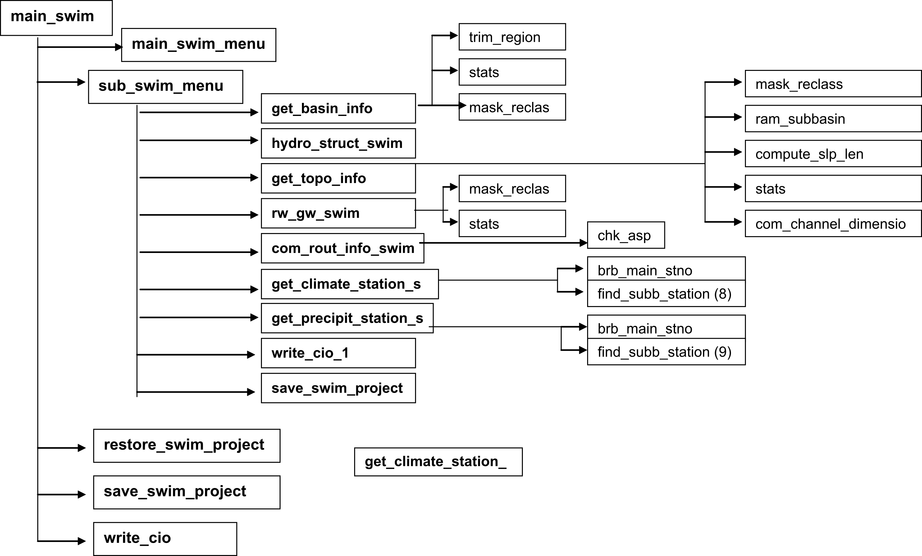
[fig:Function_tree_SWIM_GRASSinterface]
| [tab:swim_grass_interface] | ||
|---|---|---|
| Table – Continued from previous page | ||
| 1 | cell_open.c int cell_open(name,mapset) | To open an old map with name in the mapset and return the file id. To open an old map with name in the mapset and return the file id. To open an old map with name in the mapset and return the file id. |
| 2 | cell_open_new.c int cell_open_new(name) | To open an old map with name in the mapset and return the file id. |
| 3 | check_name.c int check_name(name,array,n) | To check if name corresponds to array. |
| 4 | chk_asp.c chk_asp() | To check the routing (aspect) data that was created in com_rout_info(). This will interactively allow the user to change the aspect of the basins and to store that information in proj_name.asp file under proj_name directory. It will be read by restore_project while starting the project if the status [8] is done. |
| 5 | com_rout_info_swim.c com_rout_info() | To extract routing info from basin->p, t.aspect, and temp_basin_acc maps; The information gathered will be stored in a structure which will have basin number, starting elevation, ending elevation, starting and ending accumulation cells, stream length and the next draining sub-basin number. |
| 6 | compute_slp_len.c compute_slp_len(elev_map) | To generate a slope and aspect maps from the given elevation map using the neighbourhood technique for slope prediction. It creates a new temporary map called temp_slope which has the values of slope in tenths of percent and also creates a slope length map according to the unit stream power theory. |
| 7 | display_info.c display_info() | An option to display a raster map, a site map, a vector map, to display basin number, and to restore the screen |
| 8 | dummy_lcra.c dummy_data() | dummy data for .cod file (not used in SWIM) |
| 9 | find_subb_stations.c find_subb_stations() | This subroutine establishes correspondence between sub-basins and climate/precipitation stations. |
| 10 | forms.c form1() | Forms to fill in (variant SWRRB, not used in SWIM) |
| 11 | get_basin_info.c get_basin_info() | This subroutine requests/extracts a basin information from user or from user supplied layer. |
| 12 | get_climate_station_s.c get_climate_station() | This subroutine extracts the numbers of nearest 3 climate stations for a basin or each sub-basin using program brb_main_stationno.c. The climate station number list has to be stored in a file under the active directory. The station number(s) is (are) stored in climstat_3.dat under full_path. A label file called proj_name.climstat_3 is defined which can be used to mark the stations in a map. |
| 13 | get_crop_info.c get_crop_info() | This subroutine requests/extracts the crop properties from user supplied land use map. Each sub-basin is masked and the dominant land use name is selected then the findcrop routine is called to write out the land use properties in the needed format (SWAT version, not used in SWIM). |
| 14 | get_irr_nutrient_info.c get_irr_nutrient_info() | This automatically creates .mco file for each sub-basin depending on the user’s choice for auto fertilizer and auto irrigation (SWAT variant, not used in SWIM). |
| 15 | get_mapset.c char *get_mapset(name) | To return the mapset of the map layer with the name. name: Name of the map whose mapset is needed. The mapset location is returned. |
| 16 | get_new_name.c char *get_new_name(promt,name) | To get the new map name in the current mapset using the specified prompt. It checks for the existence for the map layer with the same name and returns name, if succeeds, else quits. promt: any string to give info to the user what the program expects. name: name of the new map layer. |
| 17 | get_old_name.c char *get_old_name(prompt) | To get the old map name in any mapset using the specified prompt. It checks for the existence for the map layer and returns name, if succeeds else quits. prompt: To identify the layer one needs. |
| 18 | get_precipit_station_s.c get_pecipitation_station() | This subroutine extracts the number of nearest 3 precipitation stations for a basin or each sub-basin using program brb_main_stationno.c. The precipitation station number list has to be stored in a file in the active path. The station number(s) is (are) stored in prstat_3.dat under full_path. A label file called proj_name.prstat_3 is defined which can be used to mark the stations in a map. |
| 19 | get_rain_temp_info.c get_rain_temp_info() | This subroutine requests/extracts the rain gauge and temperature gauge station properties from user supplied map. From each sub-basin get the file name that is correspond to that sub-basin. The file has to be in SWAT format (not used in SWIM). |
| 20 | get_res_inflow.c get_res_inflow() | This requests/extracts reservoir, inflow and (re)compute the routing structures to create .fig file through a menu system (not used in SWIM). |
| 21 | get_soil_info.c get_soil_info() | This requests/extracts the soil properties from user supplied soils map. Each sub-basin is masked and the dominant soil name is picked and the findsoil routine is called to write out the soil properties in SWAT format (not used in SWIM). |
| 22 | get_topo_info.c get_topo_info() | This subroutine requests/extracts an elevation map from user and extracts the topological properties such as stream length and stream slope using ram.sub-basin program and average overland slope and slope length using compute_slp_len subroutine. It creates several intermediate layers like temp_LS, temp_slen, temp_sslp, and temp_slope. |
| 23 | hydro_struct_swim.c hydro_struct() | This function requests a basin map, land use map and soil map for one area, starts r.stats for these three maps, stores the output in "proj_name.str" under full_path except these where one of the first numbers is zero. |
| 24 | main_swim.c main() | Main program |
| 25 | main_swim_menu.c main_menu() | This subroutine provides the first menu to start with the SWIM/GRASS project. |
| 26 | mask_reclass.c mask_reclass(layer_name,cellnum,flag) | To create a temporary file for reclassification the cellnum into MASK layer. |
| 27 | read_basin.c read_basin() | This subroutine reads the extracted basin properties in SWIM format. The basin file are stored in "data_dir" and are read in to the SWIM variables. |
| 28 | read_cod.c read_cod() | This subroutine reads the extracted control properties in SWIM format. The basin file are stored in "data_dir" and are read in to the SWIM variables. |
| 29 | read_crop.c read_crop(num) | This subroutine reads the extracted crop properties that are stored in SWIM format by the findcrop program from user supplied crop map. The crop files are stored in "data_dir" and are read in to the SWIM variables for each sub-basin "num". |
| 30 | read_res.c read_res(num) | This subroutine reads the user specified reservoir data that are stored in SWIM format. The reservoir files are stored in "data_dir" as res_num.res and are read in to the SWIM variables for each sub-basin "num" (not used in SWIM). |
| 31 | read_rout.c read_rout(num) | This subroutine reads the extracted sub-basin routing properties in SWIM format. The basin file are stored in "data_dir" and are read in to the SWIM variables for sub-basin "num". |
| 32 | read_soil.c read_soil(num) | This subroutine reads the extracted soil properties that are stored in SWIM format by the findsoil program from user supplied soils map. The soil files are stored in "data_dir" and are read in to the SWIM variables for each sub-basin "num". |
| 33 | read_sub-basin.c read_sub-basin(num) | This subroutine reads the extracted sub-basin properties in SWIM format. The basin file are stored in "data_dir" and are read in to the SWIM variables for sub-basin "num". |
| 34 | read_weather.c read_weather() | This subroutine reads the generated weather parameters from the weath_gen program which is stored in SWAT format. The weather station was selected is the most closest station from the approximate centre of the Basin. The weather file is stored in "data_dir" and are read in to the SWAT variables for the whole basin (not used). |
| 35 | restore_swim_project.c restore_project() | This subroutine program retrieves the project status information from proj_file which is the project_name with .proj extension into appropriate variables. |
| 36 | rm_rast_map.c rm_rast_map(map) | This subroutine removes current raster map. |
| 37 | rw_gw_swim.c read_gw() | This subroutine reads the extracted groundwater properties in SWIM format. The groundwater parameter file are stored in "data_dir" and are read in to the SWIM variables. |
| 38 | save_swim_project.c save_project() | This program saves the project status information in proj_file which is the project_name with .proj extension. This program will be used at the end of each project, in order to keep track of the project status. |
| 39 | stats.c stats(layer_name, flag, stat) | This routine gets the categories, area flag: 1 - stores the output in a variables 2 - returns the cell number that has maximum occurrence 3 - returns the average value of the cell number 4 - returns the weighted average value of the cell number. |
| 40 | sub_swim_menu.c sub_menu() | This subroutine is the major menu in a loop to update the various data from either layers or user inputs This program will be used while working on a ongoing project. |
| 41 | what.c | This subroutine checks current GRASS window. |
| 42 | write_basin.c write_basin() | This subroutine writes the extracted basin properties in SWIM format. The basin file are stored in "data_dir" and are read as the SWIM variables. |
| 43 | write_cio_1.c write_cio() | This subroutines writes the extracted control properties in SWIM format. The basin file are stored in "data_dir" and are read as the SWIM variables. |
| 44 | write_cod.c write_cod() | This subroutine writes the extracted control properties in SWIM format. The basin file are stored in "data_dir" and are read as the SWIM variables. |
| 45 | write_crop.c write_crop(num,crp_fl) | This subroutine writes the extracted crop properties from crp_fl database in SWIM format. The crop files are stored in "data_dir" and are read as the SWIM variables for each sub-basin "num". |
| 46 | write_res.c write_res(num) | This subroutine writes the reservoir data provided by user in SWIM format The reservoir files are stored in "data_dir" as res_num.res and are read as the SWIM variables for each sub-basin "num". |
| 47 | write_rout.c write_rout() | This subroutine writes the extracted sub-basin routing properties in SWIM format. The basin file are stored in "data_dir" and are read as the SWIM variables for sub-basin "num". |
| 48 | write_soil.c write_soil(num) | This subroutine writes the extracted soil properties in SWIM format. The soil files are stored in "data_dir" and are read as the SWIM variables for each sub-basin "num". |
| 49 | write_sub-basin.c write_sub-basin() | This subroutine writes the extracted sub-basin properties in SWIM format. The basin file are stored in "data_dir" and are read as the SWIM variables for sub-basin "num". |
| 50 | write_weather.c | This subroutine writes the generated weather parameters from the weath_gen program and stores in SWIM format. The weather file is stored in "data_dir" and are read as the SWIM variables for the whole |
| Table – Continued from previous page | |
|---|---|
| cell_open.o\ | |
| cell_open_new.o\ | |
| check_name.o\ | |
| chk_asp.o\ | |
| com_rout_info_swim.o\ | |
| compute_slp_len.o\ | |
| display_info.o\ | |
| dummy_lcra.o\ | |
| find_subb_stations.o\ | |
| forms.o\ | |
| get_basin_info.o\ | |
| get_climate_station_s.o\ | |
| get_crop_info.o\ | |
| get_irr_nutrient_info.o\ | |
| get_mapset.o\ | |
| get_new_name.o\ | |
| get_old_name.o\ | |
| get_precipit_station_s.o\ | |
| get_rain_temp_info.o\ | |
| get_res_inflow.o\ | |
| get_soil_info.o\ | |
| get_topo_info.o\ | |
| hydro_struct_swim.o\ | |
| main_swim.o\ | |
| main_swim_menu.o\ | |
| mask_reclass.o\ | |
| read_basin.o\ | |
| read_cod.o\ | |
| read_crop.o\ | |
| read_res.o\ | |
| read_rout.o\ | |
| read_soil.o\ | |
| read_sub-basin.o\ | |
| read_weather.o\ | |
| restore_swim_project.o\ | |
| rm_rast_map.o\ | |
| rw_gw_swim.o\ | |
| save_swim_project.o\ | |
| stats.o\ | |
| sub_swim_menu.o\ | |
| what.o\ | |
| write_basin.o\ | |
| write_cio_1.o\ | |
| write_cod.o\ | |
| write_crop.o\ | |
| wwrite_res.o\ | |
| wwrite_rout.o\ | |
| wwrite_soil.o\ | |
| wwrite_sub-basin.o\ | |
| wwrite_weather.o\ | |
3.2 Structure of the SWIM Simulation Part
3.2.1 Files and their Functions
The simulation part of the model code consists of 33 files listed in . They can be subdivided regarding their main functions into the following parts:
main administrative files, representing three-level disaggregation procedure: basin - sub-basin - hydrotope,
climate data input or generation,
hydrological processes,
erosion, crop/vegetation growth and nutrient processes,
routing of water, sediments and nutrients,
administrative subroutines (common blocks, read input files, initialisation of variables, writing of results, and statistical evaluation of results).
Every file contains one or several subroutines with similar functions. Altogether there are 85 subroutines in the simulation part. General functions performed in the files are also shortly described in .
The block-scheme of the model operations is presented in . It shows the sequence of computing different processes.
The file Makefile used to compile SWIM code is given in .
| [tab:Files_and_subroutines] | |||
|---|---|---|---|
| Table – continued from previous page | |||
| 1 | main.f | main | Initialisation (calls subroutines reading input data), annual and daily loops, routing structure, and aggregation of results for the basin |
| 2 | sub-basin.f | sub-basin() | Sub-basin operations: initial conditions in hydrotopes in the first day, calls hydrotop, aggregates hydrotop outputs, and provides outputs from sub-basin for routing |
| 3 | hydrotop.f | hydrotop() | Simulation of all hydrological, vegetation and nutrient cycling processes in hydrotopes |
| 4 | cliread.f | cliread + sub2prst | Reading observed climate and hydrological data |
| 5 | clicon.f | clicon + clgen() | Generation of daily climate data from monthly statistical data |
| 6 | solt.f | solt() + snom() | Calculation of soil temperature and snow melt |
| 7 | curn.f | curno() + volq() + peakq() + tran() | Simulation of daily runoff, peak runoff rate and transmission losses for hydrotopes |
| 8 | evap.f | evap() | Calculation of soil evaporation and potential plant transpiration |
| 9 | perc.f | purk() + perc() + percrack() | Calculation of percolation and lateral subsurface flow from soil |
| 10 | gwat.f | gwmod() | Calculation of groundwater contribution to streamflow |
| 11 | eros.f | ecklsp() + ysed()+ enrsb() + orgnsed()+ psed() | Simulation of erosion processes |
| 12 | crop.f | crpmd() + operat() + growth() | Simulation of crop planting, growth and harvesting |
| 13 | veget.f | vegmd() | Simulation of non-crop vegetation |
| 14 | vegfun.f | wstress() + tstress() + npstress() + scurve() + ascrv() + adjustbe() | Special functions for crop and vegetation: water, temperature and N&P stress, CO2 adjustment of the biomass-energy ratio (alpha factor) |
| 15 | cropyld.f | cryld_brb | Calculation of crop yield for districts in Brandenburg |
| 16 | ncycle.f | ncycle() + nlch() + nuptake() + fert() | Simulation of N cycle in soil |
| 17 | pcycle.f | pcycle() + psollch() + puptake() | Simulation of P cycle in soil |
| 18 | route.f | route()+ add()+ transfer() | Calculation of water, sediment and nutrient routing |
| 19 | routfun.f | rthyd()+ rtsed()+ enrrt()+ rtorgn+ rtpsed+ ttcoefi()+ coefs()+qman | Routing functions |
| 20 | compar.f | Common parameters: dimensions | |
| 21 | common.f | Common blocks: parameters and variables | |
| 22 | open.f | open + opensub + opensoil + openstruct + closef + caps() | Opening and closing input/output files |
| 23 | readcod.f | readcod | Reading xxx.cod* and xxx.fig input files: codes for print and routing |
| 24 | readbas.f | readbas | Reading xxx.bsn and xxx.str input files: basin and calibration parameters, and hydrotope structure |
| 25 | readcrp.f | readcrp | Reading crop.dat input file |
| 26 | readsub.f | readsub | Call of readwet, reading sub-basin input files: xxxNN.sub**, xxxNN.gw, and xxxNN.rte |
| 27 | readsol.f | readsol + rflowtt() | Reading soil parameters from soilNN.dat files |
| 28 | readwet.f | readwet | Reading monthly weather statistical parameters for the basin |
| 29 | init.f | blockdata + init + initsums + initsub | Block data and initialisation of variables |
| 30 | initcrop.f | initcrop() | Initialisation of crop management parameters |
| 31 | genres.f | wr_daily, wr_month(), wr_annual | Writing daily, monthly and annual general results |
| 32 | flohyd.f | flomon() + floann + floave + crop_gis + hydro_gis | Writing monthly, annual and average annual water and N flows for selected hydrotopes; Writing crop yield and annual water flows (for hydrotopes) in the GRASS input format |
| 33 | stat.f | alpha() + gammad() + distn() + gcycl() + randn() + xmonth + xnash() | Statistical functions and criteria of fit |
| [tab:File_Makefile_to_compile_SWIMcode] | |
|---|---|
| Table – Continued from previous page | |
| OBJ= | clicon.o\ |
| cliread.o\ | |
| crop.o\ | |
| cropyld.o\ | |
| curn.o\ | |
| eros.o\ | |
| evap.o\ | |
| flohyd.o\ | |
| genres.o\ | |
| gwat.o\ | |
| hydrotop.o\ | |
| init.o\ | |
| initcrop.o\ | |
| main.o\ | |
| ncycle.o\ | |
| open.o\ | |
| pcycle.o\ | |
| perc.o\ | |
| readcod.o\ | |
| readcrp.o\ | |
| readbas.o\ | |
| readsub.o\ | |
| readsol.o\ | |
| readwet.o\ | |
| route.o\ | |
| routfun.o\ | |
| solt.o\ | |
| sub-basin.o\ | |
| stat.o\ | |
| veget.o\ | |
| vegfun.o\ | |
| f77 $(FFLAGS) $(OBJ) -lm -bloadmap:map.out -o swim | |
| f77 $(FFLAGS) -c $.f | |
| rm -f $(OBJ) swim |

[fig:scheme_simulation_operations]
3.2.2 Subroutines and their Functions
All the subroutines included in SWIM code are shortly described in . In addition, the Table indicates, where every subroutine is called.
| [tab:description_of_subroutines] | |||
|---|---|---|---|
| Table – continued from previous page | |||
| main.f | main | Main program. Calls subroutines reading input data and initialisation subroutines. Establishes annual and daily loops, and the routing structure. Aggregates results for the basin. | |
| sub-basin.f | sub-basin | Sub-basin operations: initialisation in hydrotopes, call hydrotop, aggregation of hydrotope outputs, setting lateral flows for routing | main |
| hydrotop.f | hydrotop | Simulation of all hydrological, vegetation and nutrient cycling processes in hydrotopes | sub-basin |
| cliread.f | cliread | this subroutine read climate data | main |
| sub2prst | this subroutine establishes the correspondence between sub-basins and precipitation stations | main | |
| clicon.f | clicon | this subroutine controls weather inputs | main |
| clgen() | this subroutine simulates daily solar radiation, daily precipitation, and max. and min. air temperature at the user option | clicon | |
| solt.f | solt | this subroutine estimates daily average temperature at the bottom of each soil layer | hydrotop |
| snom | this subroutine calculates daily snow melt when the average air temperature exceeds 0 degrees | sub-basin | |
| curn.f | curno() | this subroutine sets curve number parameters | hydrotop |
| volq() | this subroutine predicts daily runoff given daily precipitation and snowmelt using a modified curve number approach | hydrotop | |
| peakq() | this subroutine computes the peak runoff rate using a modification of the Rational Formula | sub-basin | |
| tran() | this subroutine computes channel transmission losses | sub-basin | |
| evap.f | evap() | this subroutine computes the amount of soil evaporation and potential plant evaporation using Ritchie’s model | hydrotop |
| perc.f | purk() | this is the master percolation component It divides each layer’s flow into 4 mm slugs and manages the routing process | hydrotop |
| perc() | this subroutine computes percolation and lateral subsurface flow from a soil layer when field capacity is exceeded - hillflow method | purk | |
| percrack | this subroutine computes percolation by crack flow | purk | |
| gwat.f | gwmod() | this subroutine estimates groundwater contribution to streamflow | sub-basin |
| eros.f | ecklsp() | this subroutine calculates K, P, and LS factors for hydrotope | hydrotop |
| ysed() | this subroutine predicts daily soil loss caused by water erosion using the Modified Universal Soil Loss Equation | sub-basin | |
| enrsb() | this subroutine computes enrichment ratio for sub-basin | sub-basin | |
| orgnsed() | this subroutine computes organic N loss with erosion | sub-basin | |
| psed() | this subroutine computes P loss with erosion | sub-basin | |
| crop.f | crpmd() | Main crop routine: calls operat() and growth() subroutines | hydrotop |
| operat | this subroutine sets crop operations: planting, harvesting, and kill | crpmd | |
| growth | this subroutine predicts daily potential growth of total crop biomass and roots and calculates the leaf area index. It incorporates residue and decays residue on ground surface. It calls subroutines wstress and tstress and adjusts daily dry matter to stress | crpmd | |
| veget.f | vegmd() | this subroutine predicts daily potential growth of total plant biomass and roots and calculates the leaf area index | hydrotop |
| vegfun.f | wstress() | this subroutine distributes potential plant transpiration through the root zone and calculates actual plant water use based on soil water availability. It estimates water stress factor for crops. | crpmd, vegmd |
| tstress() | this subroutine computes temperature stress for crop growth | growth, vegmd | |
| npstress() | this subroutine computes N & P stress factor | nuptake, puptake | |
| scurve() | S-curve function | growth, adjustbe | |
| ascrv() | S-curve function | readcrp | |
| adjustbe() | this subroutine adjusts biomass-energy ration to CO2 concentration | growth | |
| cropyld.f | cryld_brb | this subroutine calculates crop yield for districts in BRB, closed if not Brandenburg | main |
| ncycle.f | ncycle() | this subroutine calculates N cycle: daily N mineralisation and immobilisation considering fresh organic material (crop residue) and active and stable humus | hydrotop |
| nlch() | this subroutine computes nitrate leaching from soil | hydrotop | |
| nuptake() | this subroutine computes N-uptake by crops and natural plants | growth, vegmd | |
| fert() | this subroutine applies N and P specified by date and amount | hydrotop | |
| pcycle.f | pcycle | this subroutine computes P cycle: P flux between labile, active mineral and stable mineral P pools | hydrotop |
| psollch | this subroutine computes soluble P leaching | hydrotop | |
| puptake | this subroutine computes P-uptake by crops and natural vegetation | growth, vegmd | |
| route.f | route() | this subroutine controls the channel routing | main |
| add() | this subroutine adds outputs for | main | |
| transfer() | this subroutine controls the channel routing | main | |
| routfun.f | rthyd() | this subroutine routes a daily flow through a reach using a constant storage coefficient | route |
| rtsed() | this subroutine routes sediment from sub-basin to basin outlets, accounting for deposition (based on fall velocity) and degradation in stream | route | |
| enrrt() | this subroutine computes enrichment coefficient for N routing | route | |
| rtorgn | this subroutine computes organic N routing | route | |
| rtpsed | this subroutine computes P routing | route | |
| ttcoefi() | this subroutine computes travel time coeffs phi() for the simplified routing | main | |
| coefs() | this subroutine calculates routing coefficients | ttcoefi | |
| qman() | this subroutine computes flow using Manning equation | ttcoefi | |
| open.f | open | this subroutine opens main input files | main |
| opensub | this subroutine opens sub-basin input files | readsub | |
| opensoil | this subroutine opens soil data files 15 | readsol | |
| openstruct | this subroutine opens 16 - structure file | readbas | |
| closef | this subroutine closes files 11,12,13,14 | main | |
| caps() | this subroutine removes extra blanks | open, opensub, opensoil, openstruct | |
| readcod.f | readcod | this subroutine reads codes for printing, routing | main |
| readbas.f | readbas | this subroutine reads basin parameters and calibration parameters | main |
| readcrp.f | readcrp | this subroutine reads crop parameters | main |
| readsub.f | readsub | this subroutine reads sub-basin input parameters | main |
| readsol.f | readsol | this subroutine reads soil input parameters | main |
| rflowtt() | this subroutine computes return flow travel time | readsol | |
| readwet.f | readwet() | this subroutine reads monthly statistical weather parameters, provided by user | readsub |
| init.f | block data | block data | |
| init | this subroutine initialises variables in main | main | |
| initsums | this subroutine initialises variables for GIS output | main | |
| initsub | this subroutine initialises sub-basin variables | sub-basin | |
| initcrop.f | initcrop() | this subroutine initialises crop management | main |
| genres.f | wr_daily | this subroutine writes daily general results | main |
| wr_month() | this subroutine writes monthly general results | main | |
| wr_annual | this subroutine writes annual general results | main | |
| flohyd.f | flomon() | this subroutine writes monthly water and N flows for selected hydrotopes | main |
| floann | this subroutine writes annual water and N flows for selected hydrotopes | main | |
| floave | this subroutine writes average annual water and N flows for selected hydrotopes | main | |
| crop_gis | this subroutine writes crop yield for GRASS | sub-basin | |
| hydro_gis | this subroutine writes annual sums of water flows for hydrotopes (for GRASS) | sub-basin | |
| stat.f | alpha() | this subroutine computes alpha, the fraction of total rainfall that occurs during 0.5h | sub-basin, clicon |
| gammad() | this function provides numbers from gamma distribution | alpha | |
| distn() | this function computes the distance from the mean of a normal distribution | clgen | |
| gcycl() | this function cycles the random number generator | main | |
| randn() | this function provides random numbers ranging from 0. to 1. | init, readsub, gcycl, clicon, clgen, gammad | |
| xmonth | this subroutine calculates the month, given the day of the year | main | |
| xnash() | this subroutins computes criteria of fit | main |
3.2.3 Main Administrative Subroutines and the Parameter Read Part
The subroutine main performs initialisation of the simulation run by reading input data and initialising variables and parameters. It establishes annual and daily loops, and inside the daily loop it calls sequentially the sub-basin subroutine for every sub-basin to calculate all processes in sub-basin, and then routes lateral flows to the basin outlet following the routing structure file xxx.fig. The main subroutine also writes daily, monthly and annual results for the basin.
The subroutine sub-basin performs sub-basin operations: initialisation of variables for hydrotopes, calling of hydrotope subroutine, aggregation of hydrotope outputs, and setting lateral flows for routing.
The subroutine hydrotop controls simulation of all hydrological, vegetation and nutrient cycling processes in hydrotopes, by calling different related subroutines.
The structure of main, sub-basin and hydrotop subroutines is shown in the following , and . The user has to keep in mind that some of the calls are conditional, though it is not indicated in the Tables.
| Table – Continued from previous page | |||
|---|---|---|---|
| call sub-basin(icode,ihout,inum1,inum2,inum3,rnum1) | |||
| call route(icode,ihout,inum1,inum2,inum3,rnum1,nrch) | |||
| call transfer (icode,ihout,inum1,inum2,inum3) | |||
| call add (icode,ihout,inum1,inum2,inum3) | |||
| Table – Continued from previous page | ||
|---|---|---|
| call crop_gis(j,jea,k) | ||
| call hydro_gis(j,jea) | ||
| Table – Continued from previous page | ||||
|---|---|---|---|---|
| call npstress(uno3,uno3pot,uu) | ||||
| call npstress(uap,uapot,uu) | ||||
| [tab:structure_subroutines_open] | ||
|---|---|---|
| Table – Continued from previous page | ||
| open | open files | read 1 - file = file.cio call caps |
| readcod | read codes | read 2 - file = codedat read 3 - file = routin |
| readbas | read basin parameters, crop parameters and basin structure file | read 4 - file = basndat read 7 - file = struct.dat call openstruct:::
write 9 call openstruct:::
read 9 - file = strdat |
| readcrp | reads crop parameters | read 5 - file = crop.dat call ascrv() call ascrv() call ascrv() |
| readsub | reads sub-basin parameters | call opensub
call readwet read 12 - file = subdat read 13 - file = gwdat read 14 - file = routdat |
| readwet | reads weather parameters | read 11 - file = wgendat |
| readsol | reads soil parameters | call opensoil
call rflowtt() |
* for some files an internal name is indicated (e.g. routin), see for clarification
3.3 Input and Output Files
For application of the model the user has to prepare a number of input files. Regarding the way of data preparation, all the files can be subdivided into following categories:
3.3.1 catchment
| column | description | default |
|---|---|---|
| catchment_id | ||
| ecal | ||
| thc | ||
| roc2 | ||
| roc4 | ||
| cncor | ||
| sccor | ||
| tsnfall | ||
| tmelt | ||
| smrate | ||
| gmrate | ||
| bff | ||
| abf | ||
| delay | ||
| revapc | ||
| rchrgc | ||
| revapmn | ||
| station_id |
3.3.2 climate
| column | description | default |
|---|---|---|
| time | ||
| subbasin_id | ||
| tmean | ||
| tmin | ||
| tmax | ||
| precipitation | ||
| radiation | ||
| humidity |
3.3.3 crop
| column | description | default |
|---|---|---|
| icnum | ||
| cpnm | ||
| ird | ||
| be | ||
| hi | ||
| to | ||
| tb | ||
| blai | ||
| dlai | ||
| dlp1 | ||
| dlp2 | ||
| bn1 | ||
| bn2 | ||
| bn3 | ||
| bp1 | ||
| bp2 | ||
| bp3 | ||
| cnyld | ||
| cpyld | ||
| rdmx | ||
| cvm | ||
| almn | ||
| sla | ||
| pt2 | ||
| hun |
3.3.4 crop_management
| column | description | default |
|---|---|---|
| rotation_id | ||
| manag_id | ||
| name | ||
| nop | ||
| year | ||
| lu_id | ||
| idop1 | ||
| iopc1 | ||
| ncrp1 | ||
| idfe1 | ||
| fen1 | ||
| feno1 | ||
| fep1 | ||
| idop2 | ||
| iopc2 | ||
| ncrp2 | ||
| idfe2 | ||
| fen2 | ||
| feno2 | ||
| fep2 | ||
| idop3 | ||
| iopc3 | ||
| ncrp3 | ||
| idfe3 | ||
| fen3 | ||
| feno3 | ||
| fep3 | ||
| idop4 | ||
| iopc4 | ||
| ncrp4 | ||
| idfe4 | ||
| fen4 | ||
| feno4 | ||
| fep4 |
3.3.5 discharge
| column | description | default |
|---|---|---|
| time | ||
| BLANKENSTEIN |
3.3.6 hydrotope
| column | description | default |
|---|---|---|
| hydrotope_id | ||
| subbasin_id | ||
| landuse_id | ||
| soil_id | ||
| elevation | ||
| glacier_thickness | ||
| area | ||
| irrigation_user_id | ||
| output_label |
3.3.7 landuse
| column | description | default |
|---|---|---|
| landuse_id | ||
| name | ||
| icnum | ||
| type | ||
| canmx | ||
| cn2a | ||
| cn2b | ||
| cn2c | ||
| cn2d | ||
| lu_ETcor |
3.3.8 management
| column | description | default |
|---|---|---|
| user_id | ||
| name | ||
| first_year | ||
| last_year | ||
| ts | ||
| source | ||
| destination | ||
| trs_eff | ||
| irr_opt | ||
| irr_practice |
3.3.9 reservoir
| column | description | default |
|---|---|---|
| reservoir_id | ||
| subbasins_id | ||
| rsv_reservoir_name | ||
| capac_max | ||
| dead_stor | ||
| start_fill | ||
| res_active | ||
| res_activate_thresh | ||
| level_max | ||
| level_min | ||
| level_hpp | ||
| cap_hpp | ||
| efficiency | ||
| rsv_loss_seepage | ||
| rsv_gwc | ||
| rsv_evapc | ||
| rsv_start_year | ||
| rsv_start_day | ||
| rsv_mngmt | ||
| rsv_shr_withdr |
3.3.10 reservoir_monthly
| column | description | default |
|---|---|---|
| reservoir_id | ||
| month | ||
| rsv_cap_act | ||
| rsv_fill_min | ||
| rsv_dis_min_fill | ||
| rsv_dis_min_act | ||
| withdr_mon | ||
| ann_cycle |
3.3.11 reservoir_storage
| column | description | default |
|---|---|---|
| reservoir_id | ||
| storage_step | ||
| pol_l | ||
| pol_l2 | ||
| pol_a | ||
| pol_v | ||
| pol_hp |
3.3.12 soil
| column | description | default |
|---|---|---|
| soil_id | ||
| soil_file |
3.3.13 subbasin
| column | description | default |
|---|---|---|
| subbasin_id | ||
| chl | ||
| chs | ||
| chw | ||
| sl | ||
| stp | ||
| lat | ||
| chd | ||
| station_id | ||
| output_label | ||
| catchment_id |
3.3.14 subbasin_climate_grid
| column | description | default |
|---|---|---|
| subbasinID | ||
| lon | ||
| lat | ||
| weight |
3.3.15 subbasin_routing
| column | description | default |
|---|---|---|
| instruction | ||
| icd | ||
| iht | ||
| inm1 | ||
| inm2 | ||
| inm3 |
files created by SWIM/GRASS interface,
climate and hydrological data prepared by user,
soil data – standard (BÜK-1000) or created by user in the same format
standard crop database (file crop.dat is ready),
four additional files prepared by user from example files.
The following input files are prepared by SWIM/GRASS interface (see ):
file.cio – 1 file,
str.cio – 1 file,
xxx.fig – 1 file,
xxx.str – 1 file,
xxxNN.sub – M files, where M is the number of sub-basins,
xxxNN.gw – M files, where M is the number of sub-basins,
xxxNN.rte – M files, where M is the number of sub-basins.
The user has to prepare either one climate/hydrological file clim.dat, which includes all climate and hydrological data (see and ), or four files
prec.dat,
temp.dat,
radi.dat,
runoff.dat,
which include separately all precipitation, temperature, radiation, and runoff data for the basin. In addition, a file sub2prst.dat may be prepared, which indicates the correspondence between sub-basins and precipitation stations. This is especially useful in case of a large number of sub-basins.
The user has either to prepare all soil data, or to use available soil database for the Elbe, BÜK-1000, if this map is used. In addition, a file soil.cio has to be prepared or copied, which includes a list of all soil data file names.
The rest four files are the following:
xxx.cod, which includes program codes for printing;
xxx.bsn, which includes a set of basin parameters and a set of calibration parameters,
wstor.dat, which includes initial water storages for the reaches (may be all put to 0, or taken from the test model run at the end of the year), and
wgen.dat, which includes monthly climate statistics.
The monthly statistical data are used to run the weather generator. In case if real climate data are used, SWIM requires only average monthly maximum and minimum temperatures for the basin (needed for soil temperature routine). They can be calculated using an additional program wgenpar from the available climate data, taking as long series as possible. Then the calculated average monthly maximum and minimum temperatures have to be substituted into wgen.dat file.
| [tab:input_files] | |||||
|---|---|---|---|---|---|
| Unit No | Internal name | External name | read in | Description | Type |
| Table – Continued from previous page | |||||
| Unit No | Internal name | External name | read in | Description | Type |
| 1 | file.cio | file.cio | open, opensub | Control Input Output file. It contains all the input file names that are used by the model. | created by SWIM/GRASS |
| 2 | codedat | xxx.cod | readcod | This is the input control code file. In contains the number of sub-basins, the number of years of simulation, beginning year of simulation and print codes. | created by user from an example file |
| 3 | routin | xxx.fig | readcod | This is the basin configuration input file. It contains the routing commands to route and add flows through a basin. | created by SWIM/GRASS |
| 4 | basndat | xxx.bsn | readbas | This is the general basin input file. It contains a set of general basin parameters (including drainage area) and a set of parameters that can be used for calibration. | created by user from an example file |
| 7 | struct | xxx.str | readbas | This is the basin structure file. It describes sub-basins and hydrotopes by land use categories and soil types. | created by SWIM/GRASS |
| 8 | strlist | str.cio | openstruct | This is the control file for the basin structure. It contains file names to write sub-basin structure. | created by SWIM/GRASS |
| 9 | direc//strdat | Struc/subbNN.str | readbas | These are sub-basin structure files created by SWIM | created by SWIM |
| 10 | sub-prst.dat | sub-prst.dat | sub2prst | This file establishes correspondence between sub-basins and precipitation stations. | created by user |
| 5 | cropdb | crop.dat | readcrp | This is the crop data base input file. It contains crop specific parameters that are input to the model. | standard file |
| 11 | wgen.dat | wgen.dat | readwet | This is the weather generator input file. It contains monthly statistical parameters required for generating daily weather. Some of the parameters are needed by the model, even if observed weather data are used. | created by user from an example file |
| 12 | direc//subdat | Sub/xxxNN.sub | readsub | This is the general sub-basin input file. It contains general inputs specific for each sub-basin (area, land and channel slopes and lengths, etc. | created by SWIM/GRASS |
| 13 | direc//gwdat | Sub/xxxNN.gw | readsub | This is the groundwater input file. It contains shallow aquifer data, including a recession parameter, specific yield, a revap coefficient, and a deep aquifer percolation coefficient. | created by SWIM/GRASS |
| 14 | direc//routdat | Sub/xxxNN.rte | readsub | This is the sub-basin routing input file. This file contains data on channel dimensions (length, slope, width, depth, etc.) for the min channel in the sub-basin. | created by SWIM/GRASS |
| 20 | wstor.dat | wstor.dat | readsub | This file includes data on initial water storage in m3 in the reaches corresponding to the sub-basins. | created by user from an example file |
| 15 | soillist | soil.cio | opensoil | This is the control file for the soil database. It contains soil file names. | created by user or standard (BÜK-1000) |
| 16 | direct//soildat | Soil/soilNN.dat | readsol | These are soil parameter input files. They contain soil physical and chemical parameters. | created by user or standard (BÜK-1000) |
| 21 | clim.dat | clim.dat | cliread | This is climate (and) hydrological input data file. It may include all necessary climate and hydrological data, or only climate data for the basin. | created by user |
| 22 | prec.dat | prec.dat | cliread | This is precipitation input data file. It includes precipitation data from all used precipitation stations in/close to the basin. | created by user |
| 23 | temp.dat | temp.dat | cliread | This is temperature input data file. It includes temperature data from all used climate stations in/close to the basin. | created by user |
| 24 | radi.dat | radi.dat | cliread | This is radiation input data file. It includes radiation data from all used climate stations in/close to the basin. | created by user |
| 25 | runoff.dat | runoff.dat | cliread | This is hydrological input data file. It includes water discharge in the basin outlet (used for the hydrological validation). | created by user |
| Unit No | File name | Where used | Description |
|---|---|---|---|
| Table – Continued from previous page | |||
| Unit No | File name | Where used | Description |
| 31 | Res/wgen.out | readwet | Weather generator output |
| 32 | Res/rin.out | readbas, readsub, readsol | Write input parameters |
| 41 | Res/curn.out | curno, volq | specific subroutine output |
| 42 | Res/solt.out | solt | specific subroutine output |
| 43 | Res/tran.out | tran | specific subroutine output |
| 44 | Res/perc.out | purk, perc | specific subroutine output |
| 45 | Res/evap.out | evap | specific subroutine output |
| 46 | Res/crop.out | crop, cropyld | specific subroutine output |
| 47 | Res/eros.out | ecklsp, ysed, sub-basin | specific subroutine output |
| 48 | Res/nutr.prn | ncycle, sub-basin | specific subroutine output |
| 49 | Res/rout.out | ttcoefi, rtsed | specific subroutine output |
| 50 | Res/wstr.out | wstress | specific subroutine output |
| 51 | Res/htp-1.prn | subbasin | Daily water outputs for a hydrotop (chosen by user) |
| 52 | Res/htp-2.prn | subbasin | Daily water outputs for a hydrotop (chosen by user) |
| 53 | Res/htp-3.prn | subbasin | Daily water outputs for a hydrotop (chosen by user) |
| 54 | Res/htp-4.prn | subbasin | Daily water outputs for a hydrotop (chosen by user) |
| 55 | Res/htp-5.prn | vegmd | Daily water outputs for a hydrotop (chosen by user) |
| 56 | Res/htp-6.prn | vegmd | Daily water outputs for a hydrotop (chosen by user) |
| 57 | Res/htp-7.prn | vegmd | Daily water outputs for a hydrotop (chosen by user) |
| 61 | Res/subd.prn | subbasin | Daily water flow outputs for all sub-basins |
| 62 | Res/subm.prn | wr_month, wr_annual | Monthly sub-basin outputs for all sub-basins |
| 63 | Res/sub-1.prn | subbasin | Daily water outputs for a chosen sub-basin |
| 64 | Res/sub-2.prn | subbasin | Daily water outputs for a chosen sub-basin |
| 65 | Res/sub-3.prn | subbasin | Daily water outputs for a chosen sub-basin |
| 71 | Res/bad.prn | wr_daily | Daily water outputs for basin |
| 72 | Res/bam.prn | wr_month | Monthly water outputs for basin |
| 73 | Res/bay.prn | wr_annual | Annual water outputs for basin |
| 74 | Res/rch.prn | route | Reach outputs |
| 75 | Res/rvQ.prn | route | Reach outputs (from route) |
| 76 | Res/rvaddQ.prn | add | Reach outputs (from add) |
| 70 | Res/rvQ-mn.prn | main | Monthly reach outputs (from route) |
| 80 | Res/rvQ-ev.out | xnash | Evaluation of hydrological results |
| 77 | Flo/floMON.prn | flomon | Monthly water and N flows for 3 hydrotopes |
| 78 | Flo/floANN.prn | floann | Annual water and N flows for 3 hydrotopes |
| 79 | Flo/floAVE.prn | floave | Average water and N flows for 9 hydrotopes |
| 81 | Flo/fm-s1 | main, flomon | Monthly water and N flows for a chosen hydrotope |
| 82 | Flo/fm-s2 | main, flomon | Monthly water and N flows for a chosen hydrotope |
| 83 | Flo/fm-s3 | main, flomon | Monthly water and N flows for a chosen hydrotope |
| 84 | Flo/fm-s4 | main, flomon | Monthly water and N flows for a chosen hydrotope |
| 85 | Flo/fm-s5 | main, flomon | Monthly water and N flows for a chosen hydrotope |
| 86 | Flo/fm-s6 | main, flomon | Monthly water and N flows for a chosen hydrotope |
| 87 | Flo/fm-s7 | main, flomon | Monthly water and N flows for a chosen hydrotope |
| 88 | Flo/fm-s8 | main, flomon | Monthly water and N flows for a chosen hydrotope |
| 89 | Flo/fm-s9 | main, flomon | Monthly water and N flows for a chosen hydrotope |
| 91 | Flo/fa-s1 | floann | Annual water and N flows for a chosen hydrotope |
| 92 | Flo/fa-s2 | floann | Annual water and N flows for a chosen hydrotope |
| 93 | Flo/fa-s3 | floann | Annual water and N flows for a chosen hydrotope |
| 94 | Flo/fa-s4 | floann | Annual water and N flows for a chosen hydrotope |
| 95 | Flo/fa-s5 | floann | Annual water and N flows for a chosen hydrotope |
| 96 | Flo/fa-s6 | floann | Annual water and N flows for a chosen hydrotope |
| 97 | Flo/fa-s7 | floann | Annual water and N flows for a chosen hydrotope |
| 98 | Flo/fa-s8 | floann | Annual water and N flows for a chosen hydrotope |
| 99 | Flo/fa-s9 | floann | Annual water and N flows for a chosen hydrotope |
| 33 | GIS/yld-gis.out | crop_gis | Crop yield for all hydrotopes – as GRASS input |
| 34 | GIS/wat-gis.out | crop_gis | Water stress factor for hydrotopes – as GRASS input |
| 35 | GIS/tem-gis.out | crop_gis | Temperature stress factor for hydrotopes – as GRASS input |
| 36 | GIS/pre-gis.out | hydro_gis | Annual precipitation for hydrotopes – as GRASS input |
| 37 | GIS/eva-gis.out | hydro_gis | Annual evapotranspiration for hydrotopes – as GRASS input |
| 38 | GIS/run-gis.out | hydro_gis | Annual runoff for hydrotopes – as GRASS input |
| 39 | GIS/gwr-gis.out | hydro_gis | Annual groundwater recharge for hydrotopes – as GRASS input |
| 58 | Res/cryld.prn | operat | Original calculated crop yield for every year and for every hydrotope in cropland (sub-basin, soil) (considering all applied crop types) |
| 59 | Res/cryld-av.prn | main | Averaged crop yield over period a) for every soil and sub-basin, b) for every soil, and c) for the basin (considering all applied crop types) |
| 66 | Res/yld-dst.prn | cryld_brb | Distribution function for crop yield |
| 67 | Res/yldkr-1.prn | cryld_brb | Crop yield for kreise in BRB with the weighting coefficients accounting for wheat areal distribution |
| 68 | Res/yldkr-2.prn | cryld_brb | Crop yield for kreise in BRB with the weighting coefficients accounting for barley areal distribution |
3.4 Input Parameters
In this Section input parameters are described. They are arranged in accordance with the input files. Almost all files listed in are included, except files .CIO, climate and hydrological files. The files .CIO are not included, because they are created by SWIM/GRASS interface and do not need any editing. The format of the climate and hydrological input data is to a certain extent flexible, and preparation of this data is described in .
3.4.1 catchment_parameters
| name | description | defaults/unit |
|---|---|---|
| bsubcatch | False |
3.4.2 crop_parameters
| name | description | defaults/unit |
|---|---|---|
| cnum2 | 1.0 | |
| icc | 51.0 | |
| idlef | 0.0 | |
| ipo | 20.0 | |
| isba | 22.0 | |
| iwb | 36.0 | |
| iwr | 42.0 | |
| iww | 45.0 | |
| mfe | 7.0 | |
| mop | 7.0 | |
| nrotyrs | 3.0 |
3.4.3 erosion_parameters
| name | description | defaults/unit |
|---|---|---|
| chcc0 | 1.0 | |
| chxkc0 | 1.0 |
3.4.4 evapotranspiration_parameters
| name | description | defaults/unit |
|---|---|---|
| ec1 | 0.135000 | |
| ecal0 | 1.000000 | |
| thc0 | 1.000000 | |
| idvwk | 0.000000 | |
| iemeth | 0.000000 | |
| pit | 58.130001 | |
| radiation_switch | 0.000000 |
3.4.5 groundwater_parameters
| name | description | defaults/unit |
|---|---|---|
| abf0 | 0.5 | |
| gwq0 | 0.2 | |
| bff0 | 0.0 |
3.4.6 input_parameters
| name | description | defaults/unit |
|---|---|---|
| input_dir | input/ ... |
3.4.7 landuse_parameters
| name | description | defaults/unit |
|---|---|---|
| landuse_input_file | landuse.csv ... | |
| iicep | 1 |
3.4.8 management_parameters
| name | description | defaults/unit |
|---|---|---|
| management_users_input_dir | input/water_users ... | |
| management_input_file | management.csv ... | |
| bwam_module | False |
3.4.9 nutrient_parameters
| name | description | defaults/unit |
|---|---|---|
| degngrw | 0.30 | |
| degnsub | 0.30 | |
| degnsur | 0.02 | |
| degpsur | 0.02 | |
| retngrw | 15000.00 | |
| retnsub | 365.00 | |
| retnsur | 5.00 | |
| retpsur | 20.00 |
3.4.10 output_parameters
| name | description | defaults/unit |
|---|---|---|
| nns | 30 | |
| nsb | 30 | |
| nvrch | 18 | |
| nvsub | 30 | |
| output_dir | output ... | |
| output_write_interval | M | |
| output_float_format | f12.4 | |
| output_space_index_format | i6 | |
| output_default_format | csv | |
| master_logfile | swim.log ... | |
| log_stderr_level | warning | |
| log_stdout_level | info | |
| log_file_level | info |
3.4.11 reservoir_parameters
| name | description | defaults/unit |
|---|---|---|
| brsvmodule | False |
3.4.12 river_parameters
| name | description | defaults/unit |
|---|---|---|
| roc2_0 | 9.0 | |
| roc4_0 | 9.0 | |
| chnnc0 | 1.0 | |
| chwc0 | 1.0 | |
| prf | 1.0 | |
| roc1 | 0.0 | |
| roc3 | 0.0 | |
| spcon | 0.0 | |
| spexp | 1.0 | |
| storc1 | 0.5 | |
| tlgw | 0.0 | |
| tlrch | 1.0 | |
| evrch | 1.0 |
3.4.13 snow_parameters
| name | description | defaults/unit |
|---|---|---|
| tsnfall0 | 0.0 | |
| smrate0 | 1.0 | |
| gmrate0 | 10.0 | |
| prcor | 1.0 | |
| snow1 | 0.0 | |
| xgrad1 | 0.0 | |
| tgrad1 | 0.0 | |
| ulmax0 | 1.0 | |
| rnew | 0.08 | |
| tmelt0 | 0.0 | |
| bsnowmodule | True |
3.4.14 soil_parameters
| name | description | defaults/unit |
|---|---|---|
| ab | 0.02083 | |
| cnum1 | 2.0 | |
| cnum3 | 2.0 | |
| ekc0 | 1.0 | |
| icn | 0 | |
| ml | 10 | |
| psp | 0.5 | |
| rtn | 0.15 | |
| sccor0 | 1.0 | |
| stinco | 0.9 | |
| soil_input_dir | input/soils ... |
3.4.15 subbasin_parameters
| name | description | defaults/unit |
|---|---|---|
| climate_input_file | climate.csv ... | |
| brunoffdat | False | |
| discharge_input_file | discharge.csv ... | |
| tp5_default | 15.0 | |
| tp6_default | 22.0 | |
| tpnyr_default | 54.0 | |
| obmx | [31.4400005, 32.7099991, 34.5099983, 34.7299995... | |
| obmn | [7.51000023, 8.72000027, 10.3400002, 11.3199997... | |
| wim | [7.0, 7.0, 9.0, 9.0, 10.0, 10.0, 10.0, 10.0, 9.... | |
| prw | [0.0299999993, 0.589999974, 0.0599999987, 0.430... | |
| rst | [0.200000003, 0.200000003, 0.899999976, 1.29999... |
3.4.16 time_parameters
| name | description | defaults/unit |
|---|---|---|
| iyr | 2000 | |
| nbyr | 10 |
3.4.17 vegetation_parameters
| name | description | defaults/unit |
|---|---|---|
| co2ref | 0.0 | |
| co2sce | 0.0 | |
| epco | 1.0 | |
| ialpha | 0 | |
| ibeta | 0 | |
| ic3c4 | 0.0 | |
| rzmaxup | 0.0 | |
| ub | 3.065 | |
| bdormancy | False |
3.4.18 INPUT FILE - .cod
The xxx.cod file includes program codes (where xxx is the basin name given when using GRASS interface). An example of the xxx.cod input file format is presented in the following Table:
| Table – Continued from previous page | |||||||||||||
|---|---|---|---|---|---|---|---|---|---|---|---|---|---|
| nbyr | iyr | idaf | idal | lu | irch | nsim | msim | ign | ipd | prn | iiwst | isst | |
| 6 | 1983 | 1 | 365 | 64 | 1 | 4 | 4 | 5 | 1 | 0 | 1 | 1 | |
| isb1 | ih1 | isb2 | ih2 | isb3 | ih3 | isb4 | ih4 | isb5 | ih5 | isb6 | ih6 | isb7 | ih7 |
| 1 | 5 | 1 | 10 | 1 | 7 | 12 | 14 | 1 | 5 | 2 | 8 | 4 | 8 |
| isu1 | isu2 | isu3 | |||||||||||
| 0 | 0 | 0 | |||||||||||
| 0 | 1 | icurn | icursb | ||||||||||
| 0 | 1 | isolt | isosb | ||||||||||
| 0 | itran | ||||||||||||
| 0 | 1 | 5 | iperc | ipesb | ipehd | ||||||||
| 0 | 1 | 5 | ievap | ievsb | ievhd | ||||||||
| 0 | 2 | 26 | icrop | icrsb | icrso | ||||||||
| 0 | 7 | ieros | iersb | ||||||||||
| 0 | 1 | 1 | inutr | inusb | inuhd | ||||||||
| 0 | irout | ||||||||||||
| 0 | 1 | 5 | iswu | iwssb | iwshd | ||||||||
| 0 | igis | ||||||||||||
| 0 | iflom | ||||||||||||
| 0 | ifloa |
Parameters included in the .cod file are:
nbyr Number of years of simulation. It can range from 1 to 100 years. Beginning year of simulation. Usually the actual beginning year of record is used. Beginning year of simulation. Usually the actual beginning year of record is used.
nbyr Number of years of simulation. It can range from 1 to 100 years.
iyr Beginning year of simulation. Usually the actual beginning year of record is used.
idaf Beginning (julian) day of simulation. Usually equal to 1.
idal Last (julian) day of simulation. Usually equal to 365 or 366.
lu Number of subbasins in the basin. Corresponds to the subbasin map specified for SWIM/GRASS interface and can be taken from .cod file created by the interface.
irch Reach of measured water and sediment yields. Usually equal to 1 (corresponds to the subbasin in the basin outlet).
nsim Code for rainfal input, if weather generator is used as climate input (clicon). = simulated single precipitation for entire basin, = simulated multiple precipitation for entire basin.
msim Code for temperature input, if weather generator is used as climate input (clicon). = simulated single temperature for entire basin, = simulated multiple temperature for entire basin.
ign number of times to cycle random number generator (used in main). The random number generator seeds are contained in the SWIM program data statements. If IGN = 0, the simulation begins with these seeds. Setting IGN>0 allows the user to start each simulation with different seeds, if desired. Each time the generators cycle, they produce a new set of seeds. This feature is convenient for simulating several different weather sequences at a particular location.
ipd Print code for general results (in genres) (0= monthly, 1=daily, 2=yearly).
iprn Print code for rin.out and wgen.out files = print subbasin parameters in the file rin.out (from readsub), = print weather parameters in the file wgen.out (from readwet).
iwst Code for stat collection on monthly water yield = to skip statistical comparison, = to calculate statistics on the simulated water yield.
isst Code for stat collection on monthly sediments yield = to skip statistical comparison, = to calculate statistics on the simulated sediment yield.
isb1, isb2, isb3, isb4 subbasin number for hydrotope output (used in subbsin).
isb5, isb6, isb7 subbasin number for hydrotope output (used in vegmd).
ih1, ih2, ih3, ih4 hydrotope number for hydrotope output (corresponding to subbasins is1, is2, is3, and is4, used in subbsin)
ih5, ih6, ih7 hydrotope number for hydrotope output (corresponding to subbasins is5, is6, is7, used in vegmd)
isu1, isu2, isu3 subbasin number for subbasin output (used in subbasin)
icurn code = 1/0 to print or not from the subroutines curno and volq
icursb subbasin number for printing from the subroutines curno and volq
isolt code = 1/0 to print or not from the subroutine solt
isosb subbasin number for printing from the subroutine solt
itran code = 1/0 to print or not from the subroutine tran
iperc code = 1/0 to print or not from the subroutine purk()
ipesb subbasin number for printing from the subroutine purk()
ipehd hydrotope number for printing from the subroutine purk()
ievap code = 1/0 to print or not from the subroutine evap
ievsb subbasin number for printing from the subroutine evap
ievhd hydrotope number for printing from the subroutine evap
icrop code = 1/0 to print or not from the subroutine crpmd
icrsb subbasin number for printing from the subroutine crpmd
icrso soil number for printing from the subroutine crpmd
ieros code = 1/0 to print or not from the subroutines ecklsp(), ysed()
iersb subbasin number for printing from the subroutines ecklsp(), ysed()
inutr code = 1/0 to print or not from the subroutine ncycle()
inusb subbasin number for printing from the subroutine ncycle(), and for printing water and nutrient flows from subroutines flomon(), floann(), and floave()
inuhd hydrotope number for printing from the subroutine ncycle(), and initial hydrotope number for printing water and nutrient flows from subroutines flomon(), floann(), and floave(). Water and nutrient flows will be written for hydrotopes inuhd, inuhd+1, ... inuhd+8.
irout code = 1/0 to print or not from the subroutines rthyd() and rtsed()
iwstr code = 1/0 to print or not from the subroutine wstress()
iwssb subbasin number for printing from the subroutine wstress()
iwshd hydrotope number for printing from the subroutine wstress()
igis code = 1/0 to call or not crop_gis() and hydro_gis() from the subroutine subbasin. If igis = 1, crop_gis() and hydro_gis() will print crop yield and hydrological flows for GRASS input.
iflom code = 1/0 to call or not flomon() from main. If iflom = 1, monthly water and nutrient flows will be written for the subbasin inusb and the hydrotopes inuhd, ... , inuhd+8.
ifloa code = 1/0 to call or not floann() and floave() from main. If ifloa = 1, annual and average annual water and nutrient flows will be written for the subbasin inusb and the hydrotopes inuhd, ... , inuhd+8.
3.4.19 INPUT FILE - .fig
The xxx.fig file describes the basin routing structure (where xxx is the basin name given when using GRASS interface). An example of the xxx.fig input file format is presented in the following Table. The first line includes parameter names used by SWIM. The first two lines are not included in the actual files.
| icodes() | ihouts() | inum1s() | inum2s() | inum3s() | inum4s() | |
|---|---|---|---|---|---|---|
| Table – Continued from previous page | ||||||
| icodes() | ihouts() | inum1s() | inum2s() | inum3s() | inum4s() | |
| subbasin | 1 | 1 | 1 | 1 | ||
| subbasin | 1 | 2 | 2 | 2 | ||
| subbasin | 1 | 3 | 3 | 3 | ||
| subbasin | 1 | 4 | 4 | 4 | ||
| subbasin | 1 | 5 | 5 | 5 | ||
| subbasin | 1 | 6 | 6 | 6 | ||
| subbasin | 1 | 7 | 7 | 7 | ||
| subbasin | 1 | 8 | 8 | 8 | ||
| subbasin | 1 | 9 | 9 | 9 | ||
| subbasin | 1 | 10 | 10 | 10 | ||
| add | 5 | 11 | 7 | 8 | 8 | 1 |
| route | 2 | 12 | 6 | 11 | 6 | 3 |
| add | 5 | 13 | 12 | 6 | 6 | 3 |
| add | 5 | 14 | 13 | 9 | 6 | 3 |
| route | 2 | 15 | 5 | 14 | 5 | 5 |
| add | 5 | 16 | 15 | 5 | 5 | 5 |
| add | 5 | 17 | 16 | 4 | 5 | 5 |
| route | 2 | 18 | 3 | 17 | 3 | 7 |
| add | 5 | 19 | 18 | 3 | 3 | 7 |
| add | 5 | 20 | 19 | 10 | 3 | 7 |
| route | 2 | 21 | 2 | 20 | 2 | 9 |
| add | 5 | 22 | 21 | 2 | 2 | 9 |
| route | 2 | 23 | 1 | 22 | 1 | 10 |
| add | 5 | 24 | 23 | 1 | 1 | 10 |
| finish | 0 |
Parameters included in the .fig file are:
icodes() code to switch between routing subroutines = subbasin = route flow = add flows
ihouts() Hydrological Storage Location
inum1s() Subbasin No. (if subbasin), or Reach No. (if route), or Inflow hydrograph 1 (if add)
inum2s() Inflow Hydrograph (if route), or Inflow hydrograph 2 (if add)
inum3s() Subbasin No. (if add and route)
inum4s() Fractional Dimension (if add and route)
3.4.20 INPUT FILE - .bsn
The xxx.bsn file includes general basin parameters and calibration parameters (where xxx is the basin name given when using GRASS interface). An example of the xxx.bsn input file format is presented in the following Table.
| Table – Continued from previous page | |||||
|---|---|---|---|---|---|
| 1 | isc | ||||
| 0 | icn | ||||
| 0 | idlef | ||||
| 0.6 | thc | ||||
| da | p2(1) | bff | brt | ffcb | Original basin parameters |
| 574.76 | 1.000 | 1.000 | 0.500 | 0.000 | |
| cnum1 | cnum2 | cnum3 | Curve number, if icn=1 | ||
| 50. | 55. | 80. | |||
| gwq0 | abf0 | Groundwater parameters | |||
| 0.200 | 0.5 | ||||
| ekc0 | prf | spcon | spexp | Erosion parameters | |
| 1.0 | 1.000 | 0.0001 | 1.000 | ||
| snow1 | storc1 | stinco | Initial water storage | ||
| 0. | 0.5 | 0.90 | |||
| chwc0 | chxk0 | chcc0 | Channel parameters | ||
| 0.700 | 0.05 | 0.0 | |||
| roc1 | roc2 | roc3 | roc4 | Routing coefficients | |
| 0. | 3.0 | 0. | 13.0 | ||
| sccor | prcor | rdcor | Correction factors | ||
| 1.20 | 1.00 | 1.00 |
Parameters included in the .bsn file are:
isc code for saturated conductivity – read from database – calculated in SWIM from clay content, sand content and porosity using the method of Brakensiek
icn code for curve number method – modified CN-method as in SWAT, – CN = const for all soil and land use categories. In the case icn = 1 the user can set CN for conditions 1 equal to cnum1, and CN for conditions 3 equal to cnum3. The parameters cnum1 and cnum3 can be used as calibration parameters.
idlef code for taking into account day length effect on crop development – without the day length effect on crop development (as in SWAT), – with the day length effect on crop development.
thc correction factor for potential evapotranspiration on sky emissivity – without the sky emissivity factor, – with the sky emissivity factor. The user can set also thc to intermediate values in the range 0 – 1 and use this parameter for calibration.
da basin area in km2. This parameter should be taken from .bsn file produced by GRASS interface.
p2(1) rainfall correction factor, equal to the ratio of average rainfall to average annual rainfall for the gage in the basin outlet. When daily rainfall data is taken from a rain gauge located at a considerable distance from the basin, it may be necessary to use a rainfall correction factor other than one. If the difference between annual precipitation in the basin and rain gauge is known, a rainfall correction factor from 0.5 to 1.5 can be used.This parameter should be taken from .bsn file produced by GRASS interface. Usually is not used in SWIM.
bff baseflow factor for basin, is used to calc return flow travel time. The return flow travel time is then used to calculate percolation in soil from layer to layer. The bff factor is given in for different streams:
| Flow Characteristics | BFF |
|---|---|
| Perennial streams, flow >75% time | 1.00 |
| Flow 55-75% time | 0.75 |
| Flow 40-55% time | 0.50 |
| Flow 20-40% time | 0.25 |
| Ephemeral streams | 0.00 |
brt basin lag time in days. Basin lag time lags the subsurface flow. For BRT= 0 all subsurface flow reaches the sub-basin outlets on the day it occurs. Judgment is required to set BRT to as many days as subsurface flow from a precipitation event is expected to contribute to streamflow.This parameter should be taken from .bsn file produced by GRASS interface. It is not used in the current model version.
ffcb fraction of field capacity as initial water storage. This parameter should be taken from .bsn file produced by GRASS interface. It is not used in the current SWIM version.
cnum1 CN, conditions 1 for the case if icn = 1.
cnum2 CN, conditions 2 for the case if icn = 1.
cnum3 CN, conditions 3 for the case if icn = 1.
gwq0 initial groundwater flow contribution to streamflow, mm/day
abf0 alpha factor for grounwater. This parameter characterizes the groundwater recession (the rate at which groundwater flow is returned to the stream).
ekc0 soil erodibility correction factor. This parameter is used to correct all values ek() of soil erodibility obtained from soil database.
prf coefficient to estimate peak runoff in stream, used in calculation of sediment routing.
spcon rate parameter for estimation of sediment transport (between 0.0001 and 0.01).
spexp exponent for estimation of sediment transport (between 1. and 1.5).
snow1 initial snow content in the basin (mm).
storc1 initial water storage in streams correction coefficient.
stinco initial water content in the basin as a fraction of field capacity.
chwc0 coefficient to correct the channel width for all reaches. The channel width is estimated by GRASS interface.
chxk0 correction coefficient for channel USLE K factor
chcc0 correction coef. for channel USLE C factor
roc1, roc2 routing coefficients to calculate the storage time constant for the reach for the surface flow, xkm, from the initial estimation phi(10) and phi(13) based on channel length and celerity (in subroutine ttcoefi(j))
roc3, roc4 routing coefficients to calculate the storage time constant for the reach for the subsurface flow, xkm, from the initial estimation phi(10) and phi(13) based on channel length and celerity (in subroutine ttcoefi(j))
sccor correction factor for saturated conductivity (applied for all soils)
prcor correction factor for precipitation. Usually is not used in SWIM.
rdcor correction factor for the maximum plant root depth. Used in subroutine readcrp.
3.4.21 INPUT FILE - .str
The xxx.str file includes basin hydrotope structure parameters (where xxx is the basin name given when using GRASS interface), considering sub-basin, land use and soil. An example of the xxx.str input file format is presented in the following Table. The first line includes parameter names used by SWIM. The first two lines are not included in the actual files.
| j | n | k | ar() | ncell |
|---|---|---|---|---|
| Table – Continued from previous page | ||||
| j | n | k | ar() | ncell |
| 1 | 1 | 26 | 40000 | 1 |
| 1 | 2 | 12 | 120000 | 3 |
| 1 | 5 | 12 | 1160000 | 29 |
| 1 | 5 | 26 | 1760000 | 44 |
| 1 | 8 | 26 | 840000 | 21 |
| 1 | 9 | 12 | 1040000 | 26 |
| 1 | 9 | 26 | 80000 | 2 |
| 1 | 12 | 12 | 160000 | 4 |
| 1 | 12 | 26 | 40000 | 1 |
| 2 | 5 | 12 | 200000 | 5 |
| 2 | 5 | 26 | 320000 | 8 |
| 2 | 9 | 12 | 200000 | 5 |
| 2 | 12 | 12 | 80000 | 2 |
| 3 | 1 | 12 | 40000 | 1 |
| 3 | 2 | 17 | 40000 | 1 |
| 3 | 4 | 26 | 40000 | 1 |
| 3 | 5 | 12 | 760000 | 19 |
| 3 | 5 | 17 | 800000 | 20 |
| 3 | 5 | 19 | 480000 | 12 |
| 3 | 5 | 26 | 5400000 | 135 |
| 3 | 7 | 17 | 40000 | 1 |
| 3 | 7 | 26 | 40000 | 1 |
| 3 | 8 | 19 | 120000 | 3 |
| 3 | 9 | 26 | 840000 | 21 |
| 3 | 12 | 12 | 80000 | 2 |
| 4 | 1 | 26 | 80000 | 2 |
| 4 | 5 | 12 | 160000 | 4 |
| 4 | 5 | 26 | 680000 | 17 |
| 4 | 8 | 26 | 40000 | 1 |
| 4 | 9 | 26 | 80000 | 2 |
| 4 | 12 | 26 | 40000 | 1 |
| 5 | 1 | 26 | 320000 | 8 |
| 5 | 4 | 26 | 240000 | 6 |
| 5 | 5 | 19 | 40000 | 1 |
| 5 | 5 | 26 | 6560000 | 164 |
| 5 | 8 | 26 | 760000 | 19 |
| 5 | 9 | 26 | 2120000 | 53 |
| 5 | 12 | 26 | 160000 | 4 |
| 6 | 5 | 26 | 80000 | 2 |
| 6 | 8 | 26 | 40000 | 1 |
| 6 | 9 | 26 | 40000 | 1 |
| 6 | 12 | 26 | 40000 | 1 |
Parameters included in the .str file are:
j subbasin number (from SWIM/GRASS interface)
n land use category number (from SWIM/GRASS interface) n = 1 - water n = 2 - settlement n = 3 - industry n = 4 - road n = 5 - cropland n = 6 - set-aside n = 7 - grassland, extensive use (meadow) n = 8 - grassland, intensive use (pasture) n = 9 - forest mixed n = 10 - forest evergreen n = 11 - forest deciduous n = 12 - wetland nonforested n = 13 - wetland forested n = 14 - heather (grass + brushland) n = 15 - bare soil
k soil type (from SWIM/GRASS interface)
ar hydrotope area, corresponding to the hydrotope with the land use n and the soil k in the subbasin j. (from SWIM/GRASS interface)
ncell number of cells, corresponding to the hydrotope with the land use n and the soil k in the subbasin j. (from SWIM/GRASS interface)
3.4.22 INPUT FILE - sub-prst.dat
The sub-prst.dat file establishes the correspondence between sub-basins and precipitation stations in case if only one precipitation station is used for every sub-basin. It lists all sub-basins and the corresponding precipitation stations numbered from 1 to nst, where nst is the total number of precipitation stations used.
is1() subbasin No.
ip2() precip. stat No., corresponding to the subbasin is1() (chosen as the closest the the subbasin central point)
3.4.23 INPUT FILE - crop.dat
The crop.dat file provides crop/vegetation parameters for 71 crops/vegetation types, including some aggregated types of vegetation, like deciduous forest. This is the standard file. It is presented in Then lists abbreviated crop names, full crop names, and land cover categories.
| icnum | cpnm | ird | be | hi | to | tb | blai | dlai | dlp1 | dlp2 | bn1 | bn2 | bn3 | bp1 | bp2 | bp3 | cnyld | cpyld | rdmx | cvm | almn | sla | pt2 | hun | cpnm |
|---|---|---|---|---|---|---|---|---|---|---|---|---|---|---|---|---|---|---|---|---|---|---|---|---|---|
| Table – Continued from previous page | |||||||||||||||||||||||||
| 1 | AGRL | 1 | 40 | 0.5 | 25 | 8 | 5 | 0.8 | 15.05 | 50.95 | 0.044 | 0.0164 | 0.0128 | 0.0062 | 0.0023 | 0.0018 | 0.0175 | 0.0025 | 2 | 0.2 | 0 | 0 | 660.44 | 1500 | AGRL |
| 2 | ASPR | 1 | 90 | 0.8 | 35 | 10 | 4.2 | 1 | 25.23 | 40.86 | 0.062 | 0.05 | 0.04 | 0.005 | 0.004 | 0.002 | 0.07 | 0.0065 | 1.5 | 0.2 | 0 | 0 | 660.95 | 1500 | ASPR |
| 3 | BROC | 1 | 26 | 0.8 | 24 | 4 | 4.2 | 1 | 25.23 | 40.86 | 0.062 | 0.009 | 0.007 | 0.005 | 0.004 | 0.003 | 0.053 | 0.0073 | 0.7 | 0.2 | 0 | 0 | 660.95 | 1500 | BROC |
| 4 | CABG | 1 | 19 | 0.8 | 24 | 4 | 3 | 1 | 25.23 | 40.86 | 0.062 | 0.007 | 0.004 | 0.005 | 0.0035 | 0.002 | 0.027 | 0.0033 | 0.7 | 0.2 | 0 | 0 | 660.95 | 1500 | CABG |
| 5 | CANT | 1 | 30 | 0.5 | 32 | 16 | 3 | 0.6 | 15.05 | 50.95 | 0.0663 | 0.0255 | 0.0148 | 0.0053 | 0.002 | 0.0012 | 0.025 | 0.0022 | 1.3 | 0.03 | 0 | 0 | 660.39 | 1500 | CANT |
| 6 | CAUF | 1 | 21 | 0.8 | 24 | 7 | 2.5 | 1 | 25.23 | 40.86 | 0.062 | 0.007 | 0.004 | 0.005 | 0.0035 | 0.002 | 0.04 | 0.0057 | 0.7 | 0.2 | 0 | 0 | 660.95 | 1500 | CAUF |
| 7 | CELR | 1 | 27 | 0.8 | 24 | 7 | 2.5 | 1 | 25.23 | 40.86 | 0.062 | 0.015 | 0.01 | 0.006 | 0.005 | 0.003 | 0.022 | 0.0052 | 0.7 | 0.2 | 0 | 0 | 660.95 | 1500 | CELR |
| 8 | CORN | 1 | 40 | 0.5 | 25 | 8 | 5 | 0.8 | 15.05 | 50.95 | 0.044 | 0.0164 | 0.0128 | 0.0062 | 0.0023 | 0.0018 | 0.0175 | 0.0025 | 2 | 0.2 | 0 | 0 | 660.44 | 1500 | CORN |
| 9 | CORN | 1 | 39 | 0.55 | 35 | 8 | 3 | 0.5 | 15.05 | 50.95 | 0.047 | 0.0177 | 0.0138 | 0.0048 | 0.0018 | 0.0014 | 0.021 | 0.007 | 2 | 0.2 | 0 | 0 | 660.44 | 1500 | CORN |
| 10 | COTP | 1 | 15 | 0.4 | 27.5 | 10 | 4 | 0.95 | 15.01 | 50.95 | 0.058 | 0.0192 | 0.0177 | 0.0081 | 0.0027 | 0.0025 | 0.019 | 0.0029 | 2.2 | 0.2 | 0 | 0 | 660.19 | 1500 | COTP |
| 11 | COTS | 1 | 15 | 0.5 | 27.5 | 10 | 4 | 0.95 | 15.01 | 50.95 | 0.058 | 0.0192 | 0.0177 | 0.0081 | 0.0027 | 0.0025 | 0.014 | 0.002 | 2.2 | 0.2 | 0 | 0 | 660.19 | 1500 | COTS |
| 12 | CRRT | 1 | 30 | 1.12 | 24 | 7 | 3.5 | 0.6 | 15.01 | 50.95 | 0.055 | 0.0075 | 0.0012 | 0.006 | 0.003 | 0.002 | 0.013 | 0.0037 | 1.1 | 0.2 | 0 | 0 | 660.2 | 1500 | CRRT |
| 13 | CUCM | 1 | 30 | 0.27 | 32 | 16 | 1.5 | 0.6 | 15.05 | 50.95 | 0.0663 | 0.0075 | 0.0048 | 0.0053 | 0.0025 | 0.0012 | 0.02 | 0.0042 | 1.1 | 0.03 | 0 | 0 | 660.39 | 1500 | CUCM |
| 14 | EGGP | 1 | 30 | 0.59 | 35 | 18 | 3 | 0.6 | 15.05 | 50.95 | 0.0663 | 0.0255 | 0.0075 | 0.0053 | 0.002 | 0.0015 | 0.022 | 0.0041 | 1.1 | 0.03 | 0 | 0 | 660.39 | 1500 | EGGP |
| 15 | GRSG | 1 | 35 | 0.5 | 27.5 | 10 | 5 | 0.8 | 15.05 | 50.95 | 0.044 | 0.0164 | 0.0128 | 0.006 | 0.0022 | 0.0018 | 0.02 | 0.0028 | 2 | 0.2 | 0 | 0 | 660.38 | 1500 | GRSG |
| 16 | HMEL | 1 | 30 | 0.55 | 35 | 16 | 4 | 0.6 | 15.05 | 50.95 | 0.007 | 0.004 | 0.002 | 0.0026 | 0.002 | 0.0017 | 0.008 | 0.001 | 1.1 | 0.03 | 0 | 0 | 660.39 | 1500 | HMEL |
| 17 | ONIO | 1 | 30 | 1.25 | 29 | 7 | 1.5 | 0.6 | 15.01 | 50.95 | 0.04 | 0.03 | 0.002 | 0.0021 | 0.002 | 0.0019 | 0.021 | 0.0032 | 0.7 | 0.2 | 0 | 0 | 660.2 | 1500 | ONIO |
| 18 | PEPR | 1 | 30 | 0.6 | 27 | 18 | 5 | 0.6 | 15.05 | 50.95 | 0.06 | 0.035 | 0.025 | 0.0053 | 0.002 | 0.0012 | 0.003 | 0.002 | 1.1 | 0.03 | 0 | 0 | 660.39 | 1500 | PEPR |
| 19 | POTA | 1 | 30 | 0.95 | 18 | 7 | 5 | 0.6 | 15.01 | 50.95 | 0.055 | 0.02 | 0.012 | 0.006 | 0.0025 | 0.0019 | 0.013 | 0.002 | 2 | 0.2 | 0 | 0 | 660.2 | 1500 | POTA |
| 20 | POTA | 1 | 30 | 1.41 | 18 | 3 | 5 | 0.95 | 15.01 | 50.95 | 0.055 | 0.02 | 0.012 | 0.006 | 0.0025 | 0.0019 | 0.013 | 0.002 | 2 | 0.2 | 0 | 0 | 660.2 | 2000 | POTA |
| 21 | RICE | 1 | 25 | 0.5 | 25 | 10 | 6 | 0.8 | 30.01 | 70.95 | 0.05 | 0.02 | 0.01 | 0.006 | 0.003 | 0.0018 | 0.02 | 0.003 | 0.9 | 0.03 | 0 | 0 | 660.31 | 1500 | RICE |
| 22 | SBAR | 1 | 30 | 0.42 | 15 | 0 | 6 | 0.9 | 15.01 | 50.95 | 0.06 | 0.0231 | 0.0134 | 0.0084 | 0.0032 | 0.0019 | 0.0234 | 0.0033 | 2 | 0.01 | 0 | 0 | 660.45 | 1900 | SBAR |
| 23 | SGBT | 1 | 30 | 2 | 18 | 4 | 5 | 0.6 | 5.05 | 50.95 | 0.055 | 0.02 | 0.012 | 0.006 | 0.0025 | 0.0019 | 0.013 | 0.002 | 2 | 0.2 | 0 | 0 | 660.2 | 1500 | SGBT |
| 24 | SGHY | 1 | 35 | 0.5 | 27.5 | 10 | 5 | 0.85 | 15.01 | 50.95 | 0.044 | 0.0164 | 0.0128 | 0.006 | 0.0022 | 0.0018 | 0.02 | 0.0028 | 2 | 0.03 | 0 | 0 | 660.38 | 1500 | SGHY |
| 25 | SLMA | 1 | 60 | 1 | 20 | 5 | 8 | 0.7 | 15.05 | 50.95 | 0.044 | 0.0164 | 0.0128 | 0.0062 | 0.0023 | 0.0018 | 0.0175 | 0.0025 | 1 | 0.2 | 0 | 0 | 660.44 | 2400 | SLMA |
| 26 | SPIN | 1 | 30 | 0.95 | 24 | 4 | 4.2 | 0.95 | 10.05 | 90.95 | 0.062 | 0.04 | 0.03 | 0.005 | 0.004 | 0.0035 | 0.058 | 0.0061 | 0.7 | 0.2 | 0 | 0 | 660.95 | 1500 | SPIN |
| 27 | STRW | 1 | 30 | 0.45 | 32 | 10 | 3 | 0.6 | 15.05 | 50.95 | 0.0663 | 0.0255 | 0.0148 | 0.0053 | 0.002 | 0.0012 | 0.012 | 0.0024 | 0.7 | 0.03 | 0 | 0 | 660.39 | 1500 | STRW |
| 28 | SUGC | 1 | 25 | 0.5 | 25 | 11 | 6 | 0.75 | 15.01 | 50.95 | 0.01 | 0.004 | 0.0025 | 0.0075 | 0.003 | 0.0019 | 0 | 0 | 2 | 0.001 | 0 | 0 | 660.4 | 1500 | SUGC |
| 29 | SUNF | 1 | 35 | 0.4 | 25 | 6 | 5 | 0.55 | 15.01 | 50.95 | 0.05 | 0.023 | 0.0146 | 0.0063 | 0.0029 | 0.0023 | 0.028 | 0.0061 | 2.2 | 0.2 | 0 | 0 | 660.45 | 1500 | SUNF |
| 30 | SWHT | 1 | 30 | 0.4 | 15 | 0 | 6 | 0.8 | 15.01 | 50.95 | 0.06 | 0.0231 | 0.013 | 0.0084 | 0.0032 | 0.0019 | 0.0234 | 0.0033 | 2 | 0.03 | 0 | 0 | 660.39 | 1500 | SWHT |
| 31 | TOBC | 1 | 39 | 0.55 | 25 | 8 | 4.5 | 0.7 | 15.05 | 50.95 | 0.047 | 0.0177 | 0.0138 | 0.0048 | 0.0018 | 0.0014 | 0.014 | 0.0016 | 2 | 0.2 | 0 | 0 | 660.44 | 1500 | TOBC |
| 32 | TOMA | 1 | 30 | 0.33 | 27 | 10 | 3 | 0.95 | 15.05 | 50.95 | 0.0663 | 0.03 | 0.025 | 0.0053 | 0.0035 | 0.0025 | 0.024 | 0.0038 | 1.5 | 0.03 | 0 | 0 | 660.39 | 1500 | TOMA |
| 33 | WMEL | 1 | 30 | 0.5 | 35 | 18 | 1.5 | 0.6 | 15.05 | 50.95 | 0.0663 | 0.0075 | 0.0048 | 0.0053 | 0.0025 | 0.0012 | 0.011 | 0.0014 | 1.1 | 0.03 | 0 | 0 | 660.39 | 1500 | WMEL |
| 34 | BARL | 2 | 30 | 0.4 | 15 | 0 | 6 | 0.8 | 15.01 | 50.95 | 0.06 | 0.0231 | 0.0134 | 0.0084 | 0.0032 | 0.0019 | 0.0234 | 0.0033 | 2 | 0.03 | 0 | 0 | 660.45 | 1500 | BARL |
| 35 | BARL | 2 | 35 | 0.42 | 25 | 0 | 3.5 | 0.6 | 20.1 | 49.95 | 0.059 | 0.0226 | 0.0131 | 0.0057 | 0.0022 | 0.0013 | 0.021 | 0.0017 | 2 | 0.01 | 0 | 0 | 660.39 | 1500 | BARL |
| 36 | BARL | 2 | 30 | 0.42 | 15 | 0 | 6 | 0.9 | 15.01 | 50.95 | 0.06 | 0.0231 | 0.0134 | 0.0084 | 0.0032 | 0.0019 | 0.0234 | 0.0033 | 2 | 0.01 | 0 | 0 | 660.45 | 2300 | BARL |
| 37 | LETT | 2 | 23 | 0.8 | 18.2 | 0 | 4.2 | 1 | 25.23 | 40.86 | 0.036 | 0.025 | 0.021 | 0.0084 | 0.0032 | 0.0019 | 0.026 | 0.0049 | 0.8 | 0.01 | 0 | 0 | 660.25 | 1500 | LETT |
| 38 | LETL | 2 | 19 | 0.8 | 18.2 | 0 | 4.2 | 1 | 25.23 | 40.86 | 0.036 | 0.025 | 0.021 | 0.0084 | 0.0032 | 0.0019 | 0.026 | 0.0049 | 0.8 | 0.01 | 0 | 0 | 660.25 | 1500 | LETL |
| 39 | OATS | 2 | 30 | 0.35 | 15 | 0 | 6 | 0.8 | 15.01 | 50.95 | 0.06 | 0.0231 | 0.0134 | 0.0084 | 0.0032 | 0.0019 | 0.0234 | 0.0033 | 2 | 0.03 | 0 | 0 | 660.45 | 1500 | OATS |
| 40 | RAPE | 2 | 35 | 0.3 | 14 | 0 | 4.5 | 0.6 | 15.01 | 50.95 | 0.05 | 0.02 | 0.011 | 0.007 | 0.0025 | 0.0015 | 0.035 | 0.0067 | 2 | 0.05 | 0 | 0 | 660.4 | 1500 | RAPE |
| 41 | RYE | 2 | 35 | 0.4 | 12.5 | 0 | 6 | 0.8 | 15.01 | 50.95 | 0.06 | 0.0231 | 0.0134 | 0.0084 | 0.0032 | 0.0019 | 0.0234 | 0.0033 | 2 | 0.03 | 0 | 0 | 660.45 | 1500 | RYE |
| 42 | RYE | 2 | 35 | 0.4 | 12.5 | 0 | 6 | 0.8 | 15.01 | 50.95 | 0.06 | 0.0231 | 0.0134 | 0.0084 | 0.0032 | 0.0019 | 0.0234 | 0.0033 | 2 | 0.3 | 0 | 0 | 660.45 | 2000 | RYE |
| 43 | WHTD | 2 | 30 | 0.4 | 15 | 0 | 6 | 0.8 | 15.01 | 50.95 | 0.06 | 0.0231 | 0.013 | 0.0084 | 0.0032 | 0.0019 | 0.0209 | 0.005 | 2 | 0.03 | 0 | 0 | 660.45 | 1500 | WHTD |
| 44 | WWHT | 2 | 30 | 0.4 | 15 | 0 | 6 | 0.6 | 15.01 | 50.95 | 0.06 | 0.0231 | 0.0134 | 0.0084 | 0.0032 | 0.0019 | 0.0234 | 0.0033 | 2 | 0.03 | 0 | 0 | 660.39 | 1500 | WWHT |
| 45 | WWHT | 2 | 30 | 0.42 | 15 | 0 | 6 | 0.8 | 15.01 | 50.95 | 0.06 | 0.0231 | 0.0134 | 0.0084 | 0.0032 | 0.0019 | 0.0234 | 0.0033 | 2 | 0.03 | 0 | 0 | 660.39 | 2300 | WWHT |
| 46 | HAY | 3 | 35 | 0.01 | 25 | 12 | 5 | 0.99 | 15.01 | 50.95 | 0.06 | 0.0231 | 0.0134 | 0.0084 | 0.0032 | 0.0019 | 0.0234 | 0.0033 | 2 | 0.003 | 0 | 0 | 660.38 | 1500 | HAY |
| 47 | PAST | 3 | 35 | 0.01 | 25 | 12 | 5 | 0.99 | 15.01 | 50.95 | 0.06 | 0.0231 | 0.0134 | 0.0084 | 0.0032 | 0.0019 | 0.0234 | 0.0033 | 2 | 0.003 | 0 | 0 | 660.38 | 1500 | PAST |
| 48 | SPAS | 3 | 35 | 0.01 | 25 | 8 | 5 | 0.99 | 15.01 | 50.95 | 0.06 | 0.0231 | 0.0134 | 0.0084 | 0.0032 | 0.0019 | 0.0234 | 0.0033 | 2 | 0.003 | 0 | 0 | 660.38 | 1500 | SPAS |
| 49 | WPAS | 3 | 30 | 0.01 | 15 | 0 | 5 | 0.99 | 15.01 | 50.95 | 0.06 | 0.0231 | 0.0134 | 0.0084 | 0.0032 | 0.0019 | 0.0234 | 0.0033 | 2 | 0.003 | 0 | 0 | 660.39 | 1500 | WPAS |
| 50 | RNGB | 3 | 30 | 0.01 | 25 | 8 | 5 | 0.99 | 15.01 | 50.95 | 0.06 | 0.0231 | 0.0134 | 0.0084 | 0.0032 | 0.0019 | 0.0234 | 0.0033 | 2 | 0.003 | 0 | 0 | 660.33 | 1500 | RNGB |
| 51 | COVC | 3 | 35 | 0.01 | 25 | 8 | 5 | 0.99 | 15.01 | 50.95 | 0.06 | 0.0231 | 0.0134 | 0.0084 | 0.0032 | 0.0019 | 0.0234 | 0.0033 | 2 | 0.003 | 0 | 0 | 660.38 | 1500 | COVC |
| 52 | URBN | 3 | 8 | 0.01 | 25 | 8 | 4 | 0.99 | 15.01 | 50.95 | 0.06 | 0.0231 | 0.0134 | 0.0084 | 0.0032 | 0.0019 | 0.0234 | 0.0033 | 2 | 0.003 | 0 | 0 | 660.33 | 1500 | URBN |
| 53 | WATR | 3 | 0 | 0.01 | 25 | 8 | 0 | 0.99 | 15.01 | 50.95 | 0.06 | 0.0231 | 0.0134 | 0.0084 | 0.0032 | 0.0019 | 0.0234 | 0.0033 | 2 | 0.003 | 0 | 0 | 660.33 | 1500 | WATR |
| 54 | WETL | 3 | 30 | 0.01 | 25 | 8 | 3 | 0.99 | 15.01 | 50.95 | 0.06 | 0.0231 | 0.0134 | 0.0084 | 0.0032 | 0.0019 | 0.0234 | 0.0033 | 2 | 0.003 | 0 | 0 | 660.33 | 1500 | WETL |
| 55 | WETN | 3 | 30 | 0.01 | 25 | 8 | 3 | 0.99 | 15.01 | 50.95 | 0.06 | 0.0231 | 0.0134 | 0.0084 | 0.0032 | 0.0019 | 0.0234 | 0.0033 | 2 | 0.003 | 0 | 0 | 660.33 | 1500 | WETN |
| 56 | FRSD | 4 | 16 | 0.01 | 20 | 6 | 2 | 0.85 | 10.5 | 25.99 | 0.006 | 0.002 | 0.0015 | 0.0007 | 0.0004 | 0.0003 | 0.0015 | 0.0003 | 2 | 0.001 | 0 | 18 | 660.2 | 1500 | FRSD |
| 57 | FRSE | 4 | 16 | 0.01 | 20 | 2 | 6 | 0.85 | 10.5 | 25.99 | 0.006 | 0.002 | 0.0015 | 0.0007 | 0.0004 | 0.0003 | 0.0015 | 0.0003 | 2 | 0.001 | 1.8 | 4.5 | 660.2 | 1500 | FRSE |
| 58 | FRST | 4 | 16 | 0.01 | 20 | 2 | 5 | 0.85 | 10.5 | 25.99 | 0.006 | 0.002 | 0.0015 | 0.0007 | 0.0004 | 0.0003 | 0.0015 | 0.0003 | 2 | 0.001 | 1.2 | 11 | 660.2 | 1500 | FRST |
| 59 | FORD | 4 | 16 | 0.01 | 20 | 2 | 5 | 0.85 | 10.5 | 25.99 | 0.006 | 0.002 | 0.0015 | 0.0007 | 0.0004 | 0.0003 | 0.0015 | 0.0003 | 2 | 0.001 | 0 | 18 | 660.2 | 2500 | FORD |
| 60 | FORE | 4 | 16 | 0.01 | 20 | 2 | 3 | 0.85 | 10.5 | 25.99 | 0.006 | 0.002 | 0.0015 | 0.0007 | 0.0004 | 0.0003 | 0.0015 | 0.0003 | 2 | 0.001 | 1.8 | 4.5 | 660.2 | 2500 | FORE |
| 61 | FORM | 4 | 16 | 0.01 | 20 | 2 | 4 | 0.85 | 10.5 | 25.99 | 0.006 | 0.002 | 0.0015 | 0.0007 | 0.0004 | 0.0003 | 0.0015 | 0.0003 | 2 | 0.001 | 1.2 | 11 | 660.2 | 2500 | FORM |
| 62 | PINE | 4 | 16 | 0.75 | 20 | 2 | 5 | 0.85 | 10.5 | 25.99 | 0.006 | 0.002 | 0.0015 | 0.0007 | 0.0004 | 0.0003 | 0.0015 | 0.0003 | 2 | 0.001 | 1.8 | 4.5 | 660.2 | 1500 | PINE |
| 63 | WETF | 4 | 30 | 0.01 | 25 | 8 | 3 | 0.99 | 15.01 | 50.95 | 0.06 | 0.0231 | 0.0134 | 0.0084 | 0.0032 | 0.0019 | 0.0234 | 0.0033 | 2 | 0.003 | 1.2 | 11 | 660.33 | 1500 | WETF |
| 64 | GRBN | 5 | 25 | 0.1 | 27 | 10 | 1.5 | 0.9 | 10.05 | 80.95 | 0.004 | 0.003 | 0.0015 | 0.004 | 0.0035 | 0.0015 | 0.029 | 0.0038 | 1.1 | 0.2 | 0 | 0 | 660.34 | 1500 | GRBN |
| 65 | LIMA | 5 | 25 | 0.3 | 27 | 10 | 2.5 | 0.9 | 10.05 | 80.95 | 0.004 | 0.003 | 0.0015 | 0.0035 | 0.003 | 0.0015 | 0.036 | 0.0045 | 1.5 | 0.2 | 0 | 0 | 660.34 | 1500 | LIMA |
| 66 | PEAS | 5 | 25 | 0.3 | 27 | 7 | 2.5 | 0.6 | 10.05 | 80.95 | 0.004 | 0.003 | 0.0015 | 0.003 | 0.002 | 0.0015 | 0.041 | 0.0051 | 1.1 | 0.2 | 0 | 0 | 660.34 | 1500 | PEAS |
| 67 | PNUT | 5 | 20 | 0.4 | 25 | 13.5 | 5 | 0.75 | 15.01 | 50.95 | 0.0524 | 0.0265 | 0.0258 | 0.0074 | 0.0037 | 0.0035 | 0.065 | 0.0091 | 2 | 0.2 | 0 | 0 | 660.25 | 1500 | PNUT |
| 68 | SOYB | 5 | 25 | 0.3 | 25 | 10 | 5 | 0.9 | 15.01 | 50.95 | 0.0524 | 0.0265 | 0.0258 | 0.0074 | 0.0037 | 0.0035 | 0.065 | 0.0091 | 2 | 0.2 | 0 | 0 | 660.31 | 1500 | SOYB |
| 69 | LEN1 | 6 | 20 | 0.55 | 14 | 1 | 4 | 0.9 | 15.02 | 50.95 | 0.0524 | 0.032 | 0.0286 | 0.0074 | 0.0037 | 0.0035 | 0.04 | 0.005 | 2 | 0.2 | 0 | 0 | 660.25 | 1500 | LEN1 |
| 70 | WPEA | 6 | 20 | 0.55 | 14 | 1 | 4 | 0.9 | 15.02 | 50.95 | 0.04 | 0.026 | 0.0232 | 0.007 | 0.004 | 0.003 | 0.038 | 0.005 | 2 | 0.05 | 0 | 0 | 660.25 | 1500 | WPEA |
| 71 | ALFA | 7 | 20 | 0.01 | 15 | 1 | 5 | 0.9 | 15.01 | 50.95 | 0.05 | 0.03 | 0.02 | 0.0071 | 0.0042 | 0.0028 | 0.025 | 0.0035 | 2 | 0.01 | 0 | 0 | 660.25 | 1500 | ALFA |
| [tab:Crop_abbreviated_names] | ||||
|---|---|---|---|---|
| Crop number | Abbreviated crop name | Crop seasonality identificator | Crop name | Land cover category |
| Table – Continued from previous page | ||||
| Crop number | Abbreviated crop name | Crop seasonality identificator | Crop name | Land cover category |
| 1 | AGRL | 1 | agricultural land | row crop |
| 2 | ASPR | 1 | asparagus | row crop |
| 3 | BROC | 1 | broccoli | row crop |
| 4 | CABG | 1 | cabbage | row crop |
| 5 | CANT | 1 | cantaloupe | row crop |
| 6 | CAUF | 1 | cauliflower | row crop |
| 7 | CELR | 1 | celery | row crop |
| 8 | CORN | 1 | corn for grain | row crop |
| 9 | CORN | 1 | corn for grain | row crop |
| 10 | COTP | 1 | cotton, stripped | row crop |
| 11 | COTS | 1 | cotton, picked | row crop |
| 12 | CRRT | 1 | carrot | row crop |
| 13 | CUCM | 1 | cucumber | row crop |
| 14 | EGGP | 1 | eggplant | row crop |
| 15 | GRSG | 1 | sorghum | row crop |
| 16 | HMEL | 1 | honey melon | row crop |
| 17 | ONIO | 1 | onion | row crop |
| 18 | PEPR | 1 | pepper | row crop |
| 19 | POTA | 1 | potatoes | row crop |
| 20 | POTA | 1 | potatoes | row crop |
| 21 | RICE | 1 | rice | small grain |
| 22 | SBAR | 1 | spring barley | small grain |
| 23 | SGBT | 1 | sugar beet | row crop |
| 24 | SGHY | 1 | sorghum hay | row crop |
| 25 | SLMA | 1 | silage maize | row crop |
| 26 | SPIN | 1 | spinach | row crop |
| 27 | STRW | 1 | strawberries | row crop |
| 28 | SUGC | 1 | sugarcane | row crop |
| 29 | SUNF | 1 | sunflower | row crop |
| 30 | SWHT | 1 | spring wheat | small grain |
| 31 | TOBC | 1 | tobacco | row crop |
| 32 | TOMA | 1 | tomato | row crop |
| 33 | WMEL | 1 | water melon | row crop |
| 34 | BARL | 2 | barley | small grain |
| 35 | BARL | 2 | barley | small grain |
| 36 | BARL | 2 | winter barley | small grain |
| 37 | LETT | 2 | lettuce | row crop |
| 38 | LETL | 2 | lettuce, leaf | row crop |
| 39 | OATS | 2 | oats | small grain |
| 40 | RAPE | 2 | rape | row crop |
| 41 | RYE | 2 | rye | small grain |
| 42 | RYE | 2 | winter rye | small grain |
| 43 | WHTD | 2 | durum wheat | small grain |
| 44 | WWHT | 2 | winter wheat | small grain |
| 45 | WWHT | 2 | winter wheat | small grain |
| 46 | HAY | 3 | hay | perennial grass |
| 47 | PAST | 3 | pasture | perennial grass |
| 48 | SPAS | 3 | summer pasture | perennial grass |
| 49 | WPAS | 3 | winter pasture | perennial grass |
| 50 | RNGB | 3 | range-brush | brush |
| 51 | COVC | 3 | cover crop | grass |
| 52 | URBN | 3 | urban | urban |
| 53 | WATR | 3 | water | water |
| 54 | WETL | 3 | wetland | perennial grass |
| 55 | WETN | 3 | wetland nonforested | perennial |
| 56 | FRSD | 4 | forest deciduous | woods |
| 57 | FRSE | 4 | forest evergreen | woods |
| 58 | FRST | 4 | forest | woods |
| 59 | FORD | 4 | forest deciduous | woods |
| 60 | FORE | 4 | forest evergreen | woods |
| 61 | FORM | 4 | forest mixed | woods |
| 62 | PINE | 4 | pine | woods |
| 63 | WETF | 4 | wetland forested | woods |
| 64 | GRBN | 5 | green beans | row crop |
| 65 | LIMA | 5 | lima | row crop |
| 66 | PEAS | 5 | peas | row crop |
| 67 | PNUT | 5 | peanut | row crop |
| 68 | SOYB | 5 | soybean | row crop |
| 69 | LEN1 | 6 | lentil | row crop |
| 70 | WPEA | 6 | winter peas | row crop |
| 71 | ALFA | 7 | alfalfa | perennial grass |
Parameters included in the crop.dat file are:
icnum(ic) crop number. This is a reference number only
ic crop number in the database (file crop.dat)
cpnm(ic) crop name. This is a four character name to represent the crop.
ilcc(ic) land cover category: [1] annual crop (row crop / small grain) [2] annual winter crop (row crop / small grain) [3] perennial (grass, brush, urban, water) [4] woods [5] annual legumes (row crop) [6] annual winter legumes (row crop) [7] perennial legumes (grass)
be(ic) biomass-energy ratio. This is the potential (unstressed) growth rate (including roots) per unit of intercepted photosynthetically active radiation. This parameter should be one of the last to be adjusted. Adjustments should be based on research results. This parameter can greatly change the rate of growth, incidence of stress during the season and the resultant crop yield. Care should be taken to make adjustments in the parameter only based on data with no drought, nutrient or temperature stress.
hi(ic) harvest index. This crop parameter is based on experimental data where crop stresses have been minimized to allow the crop to attain its potential. The model adjusts hi() as water stress occurs in the period near flowering.
to(ic) optimal temperature for plant growth, degrees C. This parameter is very stable for cultivars within a species. It should not be changed once it is determined for a species. Varietal or maturity type differences are accounted for by different sums of heat units.
tb(ic) base temperature for plant growth, degrees C. This parameter is very stable for cultivars within a species. It should not be changed once it are determined for a species. Varietal or maturity type differences are accounted for by different sums of heat units.
blai(ic) Maximum potential leaf area index. BLAI may need to be adjusted for drought prone regions where planting densities are much smaller or irrigated conditions where densities are much greater.
dlai(ic) Fraction of growing season when leaf area declines. The fraction of the growing season in heat units in divided by the total heat units accumulated between planting and crop maturity. If the date at which leaf area normally declines is known, one of the drought options in SWIM can be used to estimate the fraction of heat units accumulated. The estimated heat units at maximum leaf area can then be divided by the heat units at maturity to estimate the fraction of the growing season at which leaf area index start to decline.
dlp1(ic) complex number: before decimal: fraction of growing season, after decimal: max corresponding LAI. First point on optimal leaf area development curve.
dlp2(ic) complex number: before decimal: fraction of growing season, after decimal: max corresponding LAI. Second point on optimal leaf area development curve. Explanation: Two points on optimal (non-stress) leaf area development curve. Numbers before decimal are % of growing season. Numbers after decimal are fractions of maximum potential LAI. These two points are based on research results on the % of maximum leaf area at two points in the development of leaf area.
bn1(ic) nitrogen uptake parameter #1: normal fraction of N in crop biomass at emergence, kg N/kg biomass.
bn2(ic) nitrogen uptake parameter #2: normal fraction of N in crop biomass at 0.5 maturity, kg N/kg biomass.
bn3(ic) nitrogen uptake parameter #3: normal fraction of N in crop biomass at maturity, kg N/kg biomass.
bp1(ic) phosphorus uptake parameter #1: normal fraction of P in crop biomass at emergence, kg P/kg biomass.
bp2(ic) phosphorus uptake parameter #2: normal fraction of P in crop biomass at 0.5 maturity, kg P/kg biomass.
bp3(ic) phosphorus uptake parameter #3: normal fraction of P in crop biomass at maturity, kg P/kg biomass.
cnyld(ic) fraction of nitrogen in crop yield, kg N/kg yield.
cpyld(ic) fraction of phosphorus in crop yield, kg P/kg yield.
rdmx(ic) maximum plant rooting depth (m)
cvm(ic) minimum value of C factor for water erosion. This parameter should be adjusted with intercropping or no tillage simulations to reflect the added cover.
almn(ic) LAI minimum (for forest and natural perennial vegetation).
sla(ic) specific leaf area (m2/kg). It is in SWIM used for forest and natural perennial vegetation.
pt2(ic) 2nd point on radiation use efficiency curve: complex number: The value to the left of the decimal is a CO2 atmospheric concentration higher than the ambient (in units of microliters CO2/liter air, i.e. 450 or 660). The value to the right of the decimal is the corresponding biomass-energy ratio divided by 100. Typical values of the ratio are 1.1 to 1.2 for C4 crops and 1.3 to 1.4 for C3 crops. (Kimball, B.A. 1983).
3.4.24 INPUT FILE - wgen.dat
The wgen.dat file includes monthly statistical weather parameter for basin or sub-basins. An example of the wgen.dat input file is presented in the following Table. The lines 3 – 13 include 12 monthly values.
| Table – Continued from previous page | |||||||||||
|---|---|---|---|---|---|---|---|---|---|---|---|
| 45.000 | 66.000 | 54.000 | 31.770 | ||||||||
| 2.28 | 2.09 | 6.13 | 12.10 | 18.09 | 19.70 | 22.28 | 21.85 | 17.36 | 13.16 | 6.42 | 4.16 |
| -2.33 | -3.22 | .10 | 3.65 | 7.92 | 10.25 | 12.66 | 12.42 | 9.84 | 6.73 | 1.76 | .15 |
| 0.18 | 0.14 | 0.11 | 0.10 | 0.09 | 0.08 | 0.07 | 0.07 | 0.08 | 0.10 | 0.13 | 0.15 |
| 56. | 104. | 213. | 267. | 512. | 471. | 417. | 351. | 282. | 152. | 74. | 42. |
| 7. | 7. | 9. | 9. | 10. | 10. | 10. | 10. | 9. | 9. | 7. | 7. |
| 0.37 | 0.34 | 0.35 | 0.33 | 0.32 | 0.29 | 0.35 | 0.41 | 0.51 | 0.55 | 0.56 | 0.38 |
| 0.69 | 0.67 | 0.69 | 0.64 | 0.64 | 0.61 | 0.65 | 0.70 | 0.72 | 0.78 | 0.79 | 0.4577 |
| 0.00 | 0.00 | 0.00 | 0.00 | 0.00 | 0.00 | 0.00 | 0.00 | 0.00 | 0.00 | 0.00 | 0.00 |
| 2.7 | 2.6 | 2.7 | 3.2 | 4.2 | 5.0 | 4.9 | 5.0 | 3.7 | 3.2 | 3.0 | 3.0 |
| 3.3 | 3.05 | 2.54 | 2.79 | 2.54 | 3.30 | 5.08 | 5.84 | 4.57 | 4.57 | 3.81 | 3.05 |
| 2.86 | 4.07 | 3.49 | 2.19 | 1.70 | 2.02 | 2.51 | 1.84 | 2.00 | 2.90 | 2.14 | 2.04 |
The next Table describes format of the example file wgen.dat, including parameter names given above the values.
| Table – Continued from previous page | |||||||||||
|---|---|---|---|---|---|---|---|---|---|---|---|
| tp5 | tp6 | tp24 | ylt | ||||||||
| 45.000 | 66.000 | 54.000 | 31.770 | ||||||||
| 2.28 | 2.09 | 6.13 | 12.10 | 18.09 | 19.70 | 22.28 | 21.85 | 17.36 | 13.16 | 6.42 | 4.16 |
| -2.33 | -3.22 | .10 | 3.65 | 7.92 | 10.25 | 12.66 | 12.42 | 9.84 | 6.73 | 1.76 | .15 |
| 0.18 | 0.14 | 0.11 | 0.10 | 0.09 | 0.08 | 0.07 | 0.07 | 0.08 | 0.10 | 0.13 | 0.15 |
| 56. | 104. | 213. | 267. | 512. | 471. | 417. | 351. | 282. | 152. | 74. | 42. |
| 7. | 7. | 9. | 9. | 10. | 10. | 10. | 10. | 9. | 9. | 7. | 7. |
| 0.37 | 0.34 | 0.35 | 0.33 | 0.32 | 0.29 | 0.35 | 0.41 | 0.51 | 0.55 | 0.56 | 0.38 |
| 0.69 | 0.67 | 0.69 | 0.64 | 0.64 | 0.61 | 0.65 | 0.70 | 0.72 | 0.78 | 0.79 | 0.4577 |
| 0.00 | 0.00 | 0.00 | 0.00 | 0.00 | 0.00 | 0.00 | 0.00 | 0.00 | 0.00 | 0.00 | 0.00 |
| 2.7 | 2.6 | 2.7 | 3.2 | 4.2 | 5.0 | 4.9 | 5.0 | 3.7 | 3.2 | 3.0 | 3.0 |
| 3.3 | 3.05 | 2.54 | 2.79 | 2.54 | 3.30 | 5.08 | 5.84 | 4.57 | 4.57 | 3.81 | 3.05 |
| 2.86 | 4.07 | 3.49 | 2.19 | 1.70 | 2.02 | 2.51 | 1.84 | 2.00 | 2.90 | 2.14 | 2.04 |
Parameters included in the wgen.dat file are:
tp5(j) 10 year frequency of 0.5 h rainfall (mm). Maybe basin- or subbasin-specific.
tp6(j) 10 year frequency of 6.0 h rainfall (mm). Maybe basin- or subbasin-specific.
tp24(j) Number of years of records for estimating max 0.5 h rainfall. Maybe basin- or subbasin-specific.
ylt(j) latitude of the basin or subbasin centre
obmx(mo,j) average monthly maximum air temperature, degree C.
onmn(mo,j) average monthly minimum air temperature, degree C.
cvt(mo,j) coefficient of variation for monthly temperature
obsl(mo,j) monthly average of daily solar radiation (ly)
wim monthly maximum 0.5 h rainfall (mm) for the period of record
prw(1,mo,j) monthly probability of wet day after dry day.
prw(2,mo,j) monthly probability of wet day after dry day.
wvl(mo,j) monthly number days of precipitation in a month.
rst(mo,1,j) monthly mean event of daily rainfall.
rst(mo,2,,j) monthly standard deviation of daily rainfall.
rst(mo,3,,j) monthly skew coefficient of daily rainfall.
3.4.25 INPUT FILE - .sub
The xxxNN.sub file includes sub-basin parameters (where xxx is the basin name given when using GRASS interface, NN is the sub-basin number -1). An example of the xxxNN.sub input file format is presented in the following Table.
| 0.006 | 0.000 | 0.150 | 0.000 | 3.785 | 0.002 | 2.494 | 0.370 | 0.075 | 0.150 |
| 0.000 | 500.000 | 0.500 | 104.573 | 0.007 |
The next Table describes format of the example file xxxNN.sub , including parameter names given above the values.
| flu(j) | dum | salb(j) | sno(j) | chl(1,j) | chs(j) | chw(1,j) | chk(1,j) | chn(j) | ovn(j) |
| 0.006 | 0.000 | 0.150 | 0.000 | 3.785 | 0.002 | 2.494 | 0.370 | 0.075 | 0.150 |
| rt(j) | css(j) | ecp(j) | sl(j) | stp(j) | |||||
| 0.000 | 500.000 | 0.500 | 104.573 | 0.007 |
Parameters included in the xxxNN.sub file are:
flu(j) fraction of subbasin area in the whole basin
salb(j) soil albedo.
sno(j) initial water content of snow (mm). For long term simulations the water content of snow on the ground at the beginning of simulation, SNO is usually not known, but in most cases the estimate is not critical after the first year. If a measured value of SNO is available at the beginning of the simulation, it should be used.
chl(1,j) main channel length (km). The channel length is the distance along the channel from the sub-basin outlet to the most distant point in the sub-basin. It is estimated from a topographic map by GRASS interface and used to calculate the sub-basin time of concentration.
chs(j) main channel slope (m/m). The average channel slope is computed by dividing the difference in elevation between the sub-basin outlet and the most distant point in the sub-basin. It is estimated from a topographic map by GRASS interface and used to calculate the sub-basin time of concentration.
chw(1,j) average width of main channel (m). It is estimated from a topographic map by GRASS interface. Not used by the current model version.
chk(1,j) effective hydraulic conductivity in channel alluvium (mm/hr). It is set to a default value of 0.37 by GRASS Interface. Not used by the current model version.
chn(j) Channel N value. The channel "n" value is Mannings’s "n" value. It is set to a default value 0.075 by GRASS interface and used to calculate the sub-basin time of concentration. This value may be corrected by user.
ovn(j) Overland flow N value. The surface roughness factor is Manning’s "n" values. It is set to a default value 0.150 by GRASS interface and used to calculate the sub-basin time of concentration. This value may be corrected by user. The following Tab. 3.15 contains suggested values of Manning’s "n" for various condition.
| Overland Flow | Value Chosen | Range |
|---|---|---|
| Fallow, no residue | 0.0100 | 0.008-0.012 |
| Conventional tillage, no residue | 0.0900 | 0.06-0.12 |
| Conventional tillage, residue | 0.1900 | 0.16-0.22 |
| Chisel plow, no residue | 0.0900 | 0.06-0.12 |
| Chisel plow, residue | 0.1300 | 0.10-0.16 |
| Fall disking, residue | 0.4000 | 0.30-0.50 |
| No-till, no residue | 0.0700 | 0.04-0.10 |
| No-till, (0.5-1.0 t/ha) | 0.1200 | 0.07-0.17 |
| No-till (2.0-9.0 t/ha) | 0.3000 | 0.17-0.47 |
| Rangeland (20% cover) | 0.6000 | 0.40-0.70 |
| Short grass prairie | 0.1500 | 0.10-0.20 |
| Dense grass | 0.2400 | 0.17-0.30 |
| Bermuda grass | 0.4100 | 0.30-0.48 |
rt(j) Return flow travel time(days). Return flow travel time is required for subsurface flow from the centroid of the sub-basin to reach the sub-basin outlet. The value of RT is input for each sub-basin by the SWIM user, or can be calculated by SWIM if rt=0.0 from soil hydraulic properties and flow characteristics. Experienced hydrologists familiar with the base flow characteristics of watersheds within a region should have little problem assigning reasonable values to RT. However, if the user is not familiar with the watershed, SWIM will estimate RT based on the soil’s saturated conductivity and a parameter called the baseflow factor.
css(j) Sediment concentration in return flow (ppm). Sediment concentration in return flow is usually very low and does not contribute significantly to total sediment yields unless return flow is very high. Unless the user is aware of unusual situations where CSS is extremely high, a value of [500.] ppm is a good estimate and will yield realistic results.
ecp(j) USLE erosion control practice factor P. Values of the USLE erosion control practice factor provided by Wischmeier and Smith are contained in .
| Land Slope (%) | P Value | Max length* (ft.) |
|---|---|---|
| 1 to 2 | 0.60 | 400 |
| 3 to 5 | 0.50 | 300 |
| 6 to 8 | 0.50 | 200 |
| 9 to 12 | 0.60 | 120 |
| 13 to 16 | 0.70 | 80 |
| 17 to 20 | 0.80 | 60 |
| 21 to 25 | 0.90 | 50 |
sl(j) Average slope length (m). The average slope length is estimated for each sub-basin with the Contour Extreme Point Method (Williams and Berndt, 1977).
stp(j) Average slope steepness (m/m)-
rsdin(j) Initial residue cover (kg/ha). The RSDIN is the initial residue cover at the start of simulation
3.4.26 INPUT FILE - .gw
The xxxNN.gw file includes groundwater parameters (where xxx is the basin name given when using GRASS interface, NN is the sub-basin number -1). An example of the xxxNN.gw input file format is presented in the following Table.
| 1.0000 | 0.5000 | 0.0480 | 0.0030 | 200.0000 | 0.2000 | 0.0500 | 0.0000 |
The next Table describes the format of the example file xxxNN.gw, including parameter names given above the values.
| gwht(j) | gwq(j) | abf(j) | syld(j) | delay(j) | revapc(j) | rchrgc(j) | revapmn(j) |
| 1.0000 | 0.5000 | 0.0480 | 0.0030 | 200.0000 | 0.2000 | 0.0500 | 0.0000 |
Parameters included in the xxxNN.gw file are:
gwht(j) Initial groundwater height (m)
gwq(j) Initial groundwater flow contribution to streamflow (mm/day)
In SWIM: gwq(j) = gwq0
abf(j) alpha factor for groundwater. ABF characterizes the groundwater recession and the rate at which groundwater flow is returned to the stream.
In SWIM: abf(j) = abf0
syld(j) Specific yield
delay(j) groundwater delay (days). The time it takes for water leaving the bottom of the root zone until it reaches the shallow aquifer where it can become groundwater flow.
In SWIM: delay(j) = exp(-1./(delay(i)+1.e-6))
revapc(j) Revap coefficient (0-1) is the fraction of recharge (root zone percolation) that goes to REVAP. The amount of evaporation from the shallow aquifer is determined by multiplying potential ET by REVAPC.
rchrgc(j) Deep aquifer percolation coefficient (0-1). The amount of water that percolates into the deep aquifer (from the shallow aquifer) is determined by multiplying root zone percolation by RCHRGC.
revapmn(j) Revap storage (mm). Shallow aquifer storage must exceed REVAPMN before groundwater flow can begin.
3.4.27 INPUT FILE - .rte
The xxxNN.rte file includes channel routing parameters (where xxx is the basin name given when using GRASS interface, NN is the sub-basin number -1). An example of the xxxNN.rte input file format is presented in the following Table.
| 19.447 | 0.793 | 0.002 | 3.785 | 0.050 | 1.000 | 0.280 | 1.000 |
| chw(2,j) | chd(j) | chss(j) | chl(2,j) | chnn(j) | chk(2,j) | chxk(j) | chc(j) |
| 19.447 | 0.793 | 0.002 | 3.785 | 0.050 | 1.000 | 0.280 | 1.000 |
Parameters included in the xxxNN.rte file are:
chw(2,j) Average channel width (m). It is estimated from a topographic map by GRASS interface and used for routing. May be substituted by actual channel width if available.
chd(j) Average channel depth (m). If detailed channel cross section data is unavailable, this parameter is estimated from a topographic map by GRASS interface and used for routing. May be substituted by actual channel depth if available.
chss(j) Channel slope (m/m). If detailed channel cross section data is unavailable, this parameter is estimated from a topographic map by GRASS interface and used for routing. May be substituted by actual channel slope if available.
chl(2,j) Channel length (km). If detailed channel data is unavailable, this parameter is estimated from a topographic map by GRASS interface and used for routing. May be substituted by actual channel length if available.
chnn(j) Channel n value (mm/hr). The channel "n" value is Mannings’ "n" value. It is set to a default value 0.050 (as for natural streams with few trees, stones and brush) by GRASS interface and used to calculate routing. This value may be corrected by user. The typical values of chnn() are given in for different streams.
| [tab:Values_Manningsforchannels] | ||
|---|---|---|
| Table – Continued from previous page | ||
| Channel Flow | Value Chosen | Range |
| Earth, straight and uniform | 0.0250 | 0.016-0.033 |
| Earth, winding and sluggish | 0.0350 | 0.023-0.05 |
| Not maintained, weeds and brush | 0.0750 | 0.04-0.14 |
| Few trees, stones, or brush | 0.0500 | 0.025-0.065 |
| Heavy timber and brush | 0.1000 | 0.05-0.15 |
chk(2,j) Effective hydraulic conductivity in channel alluvium (mm/hr). It is set to a default value 1.0 (as for very low loss rate) by GRASS interface and used to calculate routing. This value may be corrected by user. Effective hydraulic conductivity of the channel alluvium is given in for various channel bed material.
| Bed Material Group | Bed Material Characteristics | Effective Hydraulic Conductivity (mm/hr) |
|---|---|---|
| Table – Continued from previous page | ||
| Bed Material Group | Bed Material Characteristics | Effective Hydraulic Conductivity (mm/hr) |
| 1 Very high loss rate | Very clean gravel and large sand d50>2 mm | >127 |
| 2 High loss rate | Clean sand and gravel under field conditions, d50>2 mm | 51-127 |
| 3 Moderate high loss rate | Sand and gravel mixture with less than a few percent silt-clay | 25-76 |
| 4 Moderate loss rate | Mixture of sand and gravel with significant amounts of silt-clay | 6.4-25 |
| 5 Very low loss rate | Consolidated bed material with high silt-clay content | 0.025-2.5 |
chxk(j) erodibility of stream channel, or USLE soil factor K for channel (range: 0-1). chxk=0 indicates a nonerosive channel, while chxk = 1 indicates no resistance to erosion. It is set to a default value 0.28 by GRASS interface and used in calculating routing. This value may be corrected by user.
chc(j) Cover factor for stream channel, or USLE soil factor C for channel (range: 0-1). If there is no vegatative cover, chc = 1. It is set to a default value of 1.0 (no vegetative cover) by GRASS interface and used to calculate routing. This value may be corrected by user.
3.4.28 INPUT FILE - wstor.dat
The wstor.dat file sets initial storage values for the reaches. It lists all reaches and the corresponding initial water storage in m3. The values for initialisation can be obtained from a test run, considering the simulated water storage at the end of the first year.
i1 reach, corresponding to the subbasin i1
sdtsav initial water storage in the reach i1
3.4.29 INPUT FILE - soilNN.dat
The soilNN.dat files include soil parameters (where, NN is the soil type number). An example of the soilNN.dat input file format is presented in the following Table.
| Table – Continued from previous page | ||||
|---|---|---|---|---|
| 36 | 5 | |||
| Ap | Ap Ahl | AhBt | Bt | |
| Ut3 | Ut3 | Ut3 | Lu | Ut3 |
| 10. | 300.0 | 600.0 | 1000.0 | 1100.0 |
| 15. | 15. | 15. | 25. | 15. |
| 75. | 75. | 75. | 60. | 75. |
| 10. | 10. | 10. | 15. | 10. |
| 1.40 | 1.40 | 1.50 | 1.70 | 1.6 |
| 52.5 | 52.5 | 50.5 | 45.5 | 40.5 |
| 26.5 | 26.5 | 26. | 17.5 | 23.5 |
| 41.5 | 41.5 | 40. | 39. | 36. |
| 2.0 | 2.0 | 1.2 | 0.9 | 0. |
| 0.2 | 0.2 | 0.1 | 0. | 0.0 |
| 0.56 | ||||
| 16.7 | 16.7 | 10.4 | 4.2 | 10.4 |
| Table – Continued from previous page | ||||
|---|---|---|---|---|
| k | ns(k) | |||
| 36 | 5 | |||
| Ap | Ap Ahl | AhBt | Bt | |
| Ut3 | Ut3 | Ut3 | Lu | Ut3 |
| 10. | 300.0 | 600.0 | 1000.0 | 1100.0 |
| 15. | 15. | 15. | 25. | 15. |
| 75. | 75. | 75. | 60. | 75. |
| 10. | 10. | 10. | 15. | 10. |
| 1.40 | 1.40 | 1.50 | 1.70 | 1.6 |
| 52.5 | 52.5 | 50.5 | 45.5 | 40.5 |
| 26.5 | 26.5 | 26. | 17.5 | 23.5 |
| 41.5 | 41.5 | 40. | 39. | 36. |
| 2.0 | 2.0 | 1.2 | 0.9 | 0. |
| 0.2 | 0.2 | 0.1 | 0. | 0.0 |
| 0.56 | ||||
| 16.7 | 16.7 | 10.4 | 4.2 | 10.4 |
Parameters included in the soilNN.dat file are:
k soil type number in a database
ns(k) number of soil layers for soil k. Number of soil layers for soil. The number of soil layers is assigned by the user. Usually the depths to the bottom of the layers are assigned in accordance with available database. Up to 10 layers are allowed, the first layer should be a depth of 10 mm.
snam(k) name of soil k
z(l,k) depth to bottom of layers l=1,...,ns(k) in mm
cla(l,k) clay content in %
sil(l,k) silt content %
san(l,k) sand content, %
por(l,k) bulk density (g/cm3) (input), then recalculated to porosity
poros(l,k) porosity, % (if available). If available water capacity, field capacity or total porosity values are missing, they can be estimated based on texture as in .
awc(l,k) available water capacity, %. If available water capacity, field capacity or total porosity values are missing, they can be estimated based on texture as in .
fc(l,k) field capacity, %. If available water capacity, field capacity or total porosity values are missing, they can be estimated based on texture as in .
cbn(l,k) organic carbon content (%)
wn(l,k) organic nitrogen content (%)
wno3(l,k) initial NO3-N content (kg/ha), if available. Otherwise, it will be estimated from wn().
ap(l,k) labile (soluble) phosphorus (g/t), if available. Otherwise, it will be estimated.
ek(k) soil erodibility factor K (for USLE)
sc(l,k) saturated conductivity (mm/h)
The following may be useful, if all necessary soil parameters are not available.
| Texture | Bulk Density (gm/cm) | Total Porosity | Field Capacity 1/3 bar | Wilting Point 15 bar | Available Water Capacity |
|---|---|---|---|---|---|
| Table – Continued from previous page | |||||
| Texture | Bulk Density (gm/cm) | Total Porosity | Field Capacity 1/3 bar | Wilting Point 15 bar | Available Water Capacity |
| Coarse sand | 1.6 | 0.4 | 0.11 | 0.03 | 0.08 |
| Sand | 1.6 | 0.4 | 0.16 | 0.03 | 0.13 |
| Fine sand | 1.5 | 0.43 | 0.18 | 0.03 | 0.15 |
| Very fine sand | 1.5 | 0.43 | 0.27 | 0.03 | 0.25 |
| Loamy coarse sand | 1.6 | 0.4 | 0.16 | 0.05 | 0.11 |
| Loamy sand | 1.6 | 0.4 | 0.19 | 0.05 | 0.14 |
| Loamy fine sand | 1.6 | 0.4 | 0.22 | 0.05 | 0.18 |
| Loamy very fine sand | 1.6 | 0.4 | 0.37 | 0.05 | 0.32 |
| Coarse sandy loam | 1.6 | 0.4 | 0.19 | 0.08 | 0.11 |
| Sandy loam | 1.6 | 0.4 | 0.22 | 0.08 | 0.14 |
| Fine sandy loam | 1.7 | 0.36 | 0.27 | 0.08 | 0.19 |
| Very fine sandy loam | 1.6 | 0.4 | 0.37 | 0.08 | 0.29 |
| Loam | 1.6 | 0.4 | 0.26 | 0.11 | 0.15 |
| Silt loam | 1.5 | 0.43 | 0.32 | 0.12 | 0.2 |
| Silt | 1.4 | 0.47 | 0.27 | 0.03 | 0.24 |
| Sandy clay loam | 1.6 | 0.4 | 0.3 | 0.18 | 0.12 |
| Clay loam | 1.6 | 0.4 | 0.35 | 0.22 | 0.13 |
| Silty clay loam | 1.4 | 0.47 | 0.36 | 0.2 | 0.16 |
| Sandy clay | 1.6 | 0.4 | 0.28 | 0.2 | 0.13 |
| Silty clay | 1.5 | 0.48 | 0.4 | 0.3 | 0.14 |
| Clay | 1.4 | 0.47 | 0.39 | 0.28 | 0.11 |
3.4.30 BLOCK DATA in the file init.f
Curve Numbers for 15 land use categories are initialized in block data (file init.f). The following values summarized in are assigned for land use categories and soil groups in SWIM. presents SCS runoff curve numbers for a variety of land use/land cover categories.
| Land Use No. | Land use category | Soil group A | Soil group B | Soil group C | Soil group D | Source in SCS Tables |
|---|---|---|---|---|---|---|
| Table – Continued from previous page | ||||||
| Land Use No. | Land use category | Soil group A | Soil group B | Soil group C | Soil group D | Source in SCS Tables |
| 1 | Water | 100 | 100 | 100 | 100 | |
| 2 | Settlement | 72 | 79 | 85 | 88 | Urban areas, medium density |
| 3 | Industry | 81 | 88 | 91 | 93 | Industrial |
| 4 | Road | 98 | 98 | 98 | 98 | Paved streets and roads |
| 5 | Cropland | 65 | 75 | 82 | 86 | Row crops, contoured |
| 6 | Set-aside | 66 | 77 | 85 | 89 | Rotation meadow |
| 7 | Extensive grassland (meadow) | 30 | 58 | 71 | 78 | Meadow, continuous grass |
| 8 | Intensive grassland (pasture) | 49 | 69 | 79 | 84 | Pasture, continuous forage for grazing |
| 9 | Mixed forest | 36 | 60 | 73 | 79 | Woods, fair |
| 10 | Evergreen forest | 36 | 60 | 73 | 79 | Woods, fair |
| 11 | Deciduous forest | 36 | 60 | 73 | 79 | Woods, fair |
| 12 | Wetland nonforested | 85 | 85 | 85 | 85 | |
| 13 | Wetland forested | 85 | 85 | 85 | 85 | |
| 14 | Heather (grass + brushland) | 35 | 56 | 70 | 77 | Brush-weed-grass mixture with brush the major element |
| 15 | Bare soil | 77 | 86 | 91 | 94 |
| [tab:SCS_Curve_Numbers] | ||||||
|---|---|---|---|---|---|---|
| Land Use/Crop | Cover | Condition | A | B | C | D |
| Table – Continued from previous page | ||||||
| Land Use/Crop | Cover | Condition | A | B | C | D |
| Fallow | Straight row | — | 77 | 86 | 91 | 94 |
| Poor | 72 | 81 | 88 | 91 | ||
| Good | 67 | 78 | 85 | 89 | ||
| Poor | 70 | 79 | 84 | 88 | ||
| Good | 65 | 65 | 82 | 86 | ||
| Poor | 66 | 74 | 80 | 82 | ||
| Good | 62 | 71 | 78 | 81 | ||
| Poor | 65 | 76 | 84 | 88 | ||
| Good | 63 | 75 | 83 | 87 | ||
| Poor | 63 | 74 | 82 | 85 | ||
| Good | 61 | 73 | 81 | 84 | ||
| Poor | 61 | 72 | 79 | 82 | ||
| Good | 59 | 70 | 78 | 81 | ||
| Poor | 65 | 76 | 84 | 88 | ||
| Good | 63 | 75 | 83 | 87 | ||
| Poor | 63 | 74 | 82 | 85 | ||
| Good | 61 | 73 | 81 | 84 | ||
| Poor | 61 | 72 | 79 | 82 | ||
| Good | 59 | 70 | 78 | 81 | ||
| [b 1]* Close-seeded legumes* or rotation meadow | Poor | 66 | 77 | 85 | 89 | |
| Good | 58 | 72 | 81 | 85 | ||
| Poor | 64 | 75 | 83 | 85 | ||
| Good | 55 | 69 | 78 | 83 | ||
| Poor | 63 | 73 | 80 | 83 | ||
| Good | 51 | 67 | 76 | 80 | ||
| Poor | 68 | 79 | 86 | 89 | ||
| Fair | 49 | 69 | 79 | 84 | ||
| Good | 39 | 61 | 74 | 80 | ||
| Poor | 47 | 67 | 81 | 88 | ||
| Fair | 25 | 59 | 75 | 83 | ||
| Good | 6 | 35 | 70 | 79 | ||
| Meadow | Good | 30 | 58 | 71 | 78 | |
| [6]* | Poor | 45 | 66 | 77 | 83 | |
| Fair | 36 | 60 | 73 | 79 | ||
| Good | 25 | 55 | 70 | 77 | ||
| Farmsteads | — | 59 | 74 | 82 | 86 | |
| Roads (dirt)** | — | 72 | 82 | 87 | 89 | |
| Roads (hard surface)** | — | 74 | 84 | 90 | 92 |
4 How to Prepare Data and Run SWIM
The model runs under the UNIX environment with the daily time step. The SWIM/GRASS interface is used to initialise the model by extracting spatially distributed parameters of elevation, land use, soil types, closest climate/precipitation station, and the routing structure.
The preparation to the modelling consists of the following steps:
preparation of spatial data in GRASS (described in ),
run SWIM/GRASS interface using the spatial data in GRASS (described in ), vpreparation of relational data (described in ), which includes:
climate data (in ),
soil data (),
crop management data ()
hydrological and water quality data ()
copy all input data in the working directory and modification of several data-handling routines, if necessary (described in ).
After that the model can be run. The calibration parameters and some examples of the model sensitivity studies are given in .
4.1 Spatial Data Preparation
First, an overview of necessary spatial data in given in . After that, two important questions: how the resolution of the Digital Elevation Model is related to the basin area, and how the average sub-basin area must be chosen, are discussed in and . Then a short overview of GRASS GIS is given in , and some GRASS operations, useful for spatial data preparation, are described in and . A specific program for watershed analysis r.watershed is described separately in . A DEMO data set is given in
4.1.1 GIS Data Overview
The full list of necessary spatial data (digitised maps) is the following:
Digital Elevation Model (DEM),
land use map,
soil map,
map of basin and sub-basins boundaries,
map of river network,
map of river gage stations,
alpha-factor map for groundwater,
map of climate stations,
map of Thiessen polygons for climate stations,
map of precipitation stations,
map of Thiessen polygons for precipitation stations
map of point sources of pollution.
All the maps can be provided in ARC/INFO or GRASS format.
The first four maps: DEM, land use, soil and sub-basins are absolutely necessary to run the SWIM/GRASS ínterface and initialise the model (see, for example, ).
For the DEM resolution is important (see ). The soil map has to be connected to soil parameters (see a detailed description in ). The land use map has to be reclassified for SWIM to a map with the following categories:
n = 1 - water
n = 2 - settlement n = 3 - industry n = 4 - road n = 5 - cropland n = 6 - set-aside n = 7 - grassland, extensive use (meadow) n = 8 - grassland, intensive use (pasture) n = 9 - forest mixed n = 10 - forest evergreen n = 11 - forest deciduous n = 12 - wetland nonforested n = 13 - wetland forested n = 14 - heather (grass + brushland) n = 15 - bare soil
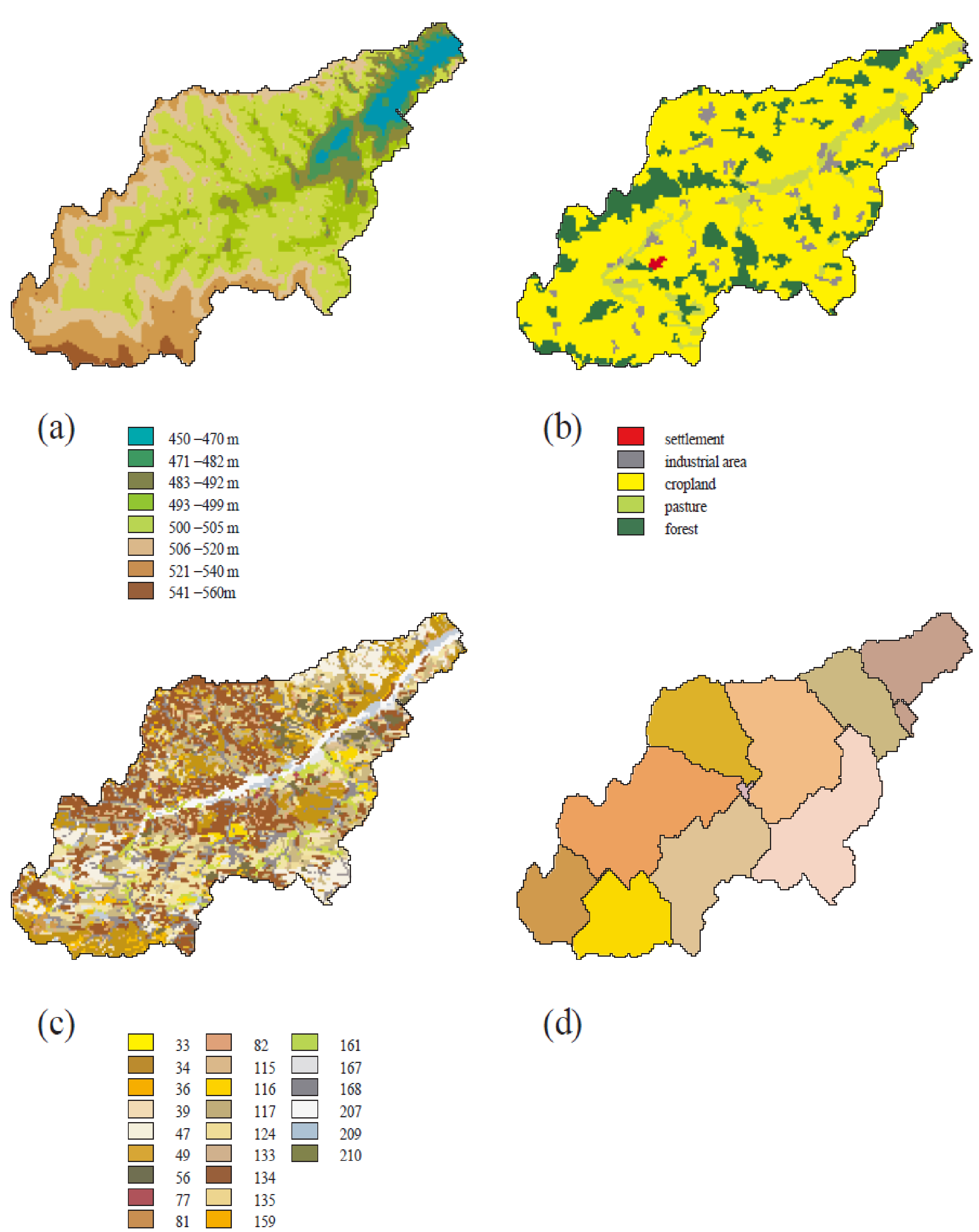
[fig:dem_landuse_soil_subbasin]
The fourth, sub-basin map, can be created in GRASS based on the DEM map using the r.watershed program. Here the DEM resolution is important (see for more details). There is a certain restriction on the average sub-basin area in SWIM, which has to be kept (see more details in ). Together with sub-basins, the virtual river network can be calculated, which is useful for checking the routing structure.
The map of river network (5) is useful for comparison with the virtual river network calculated by r.watershed, and for checking the routing structure. Comparison of river networks calculated in GRASS and digitazed is demonstrated in for the Mulde basin.
The map of river gage stations (6) can be used for delineation of the basin boundaries, if the sub-basin map is created in GRASS.
The alpha-factor map for groundwater (7) is useful, if the ground water table has to be modelled specifically for the basin under study.
Maps of climate and precipitation stations and the corresponding maps of Thiessen polygons (8-11) are more important for larger basins, having several climate/precipitation stations. For smaller basins this information can be extracted directly from available paper maps. The Thiessen polygons can be also calculated in GRASS version 4.2 using the functions s.geom or v.geom.
A map of point sources of pollution (12) is necessary in case of water quality modelling, when the simulated load is compared with the observed load, and the point sources of pollution contribute a significant part in the river load and must be taken into account.
An important question is how to choose an adequate spatial resolution for the mesoscale river basin under study. This problem is of fundamental significance for hydrological and hydrochemical process modelling.
First of all, the spatial resolution and the time increment of the model are interrelated. SWIM is not designed for detailed modelling of flood processes with T < 1 day. Also, we exclude very flat areas with many lakes, where travelling time becomes too large. These problems require specific modelling tools. With these exceptions, the problem of spatial resolution appears in at least two very important questions:
how the resolution of the Digital Elevation Model (DEM) is related to the watershed area, and
whether an upper limit of a sub-basin area exists below which the effect of the river network can be neglected.
These two questions are discussed in and .
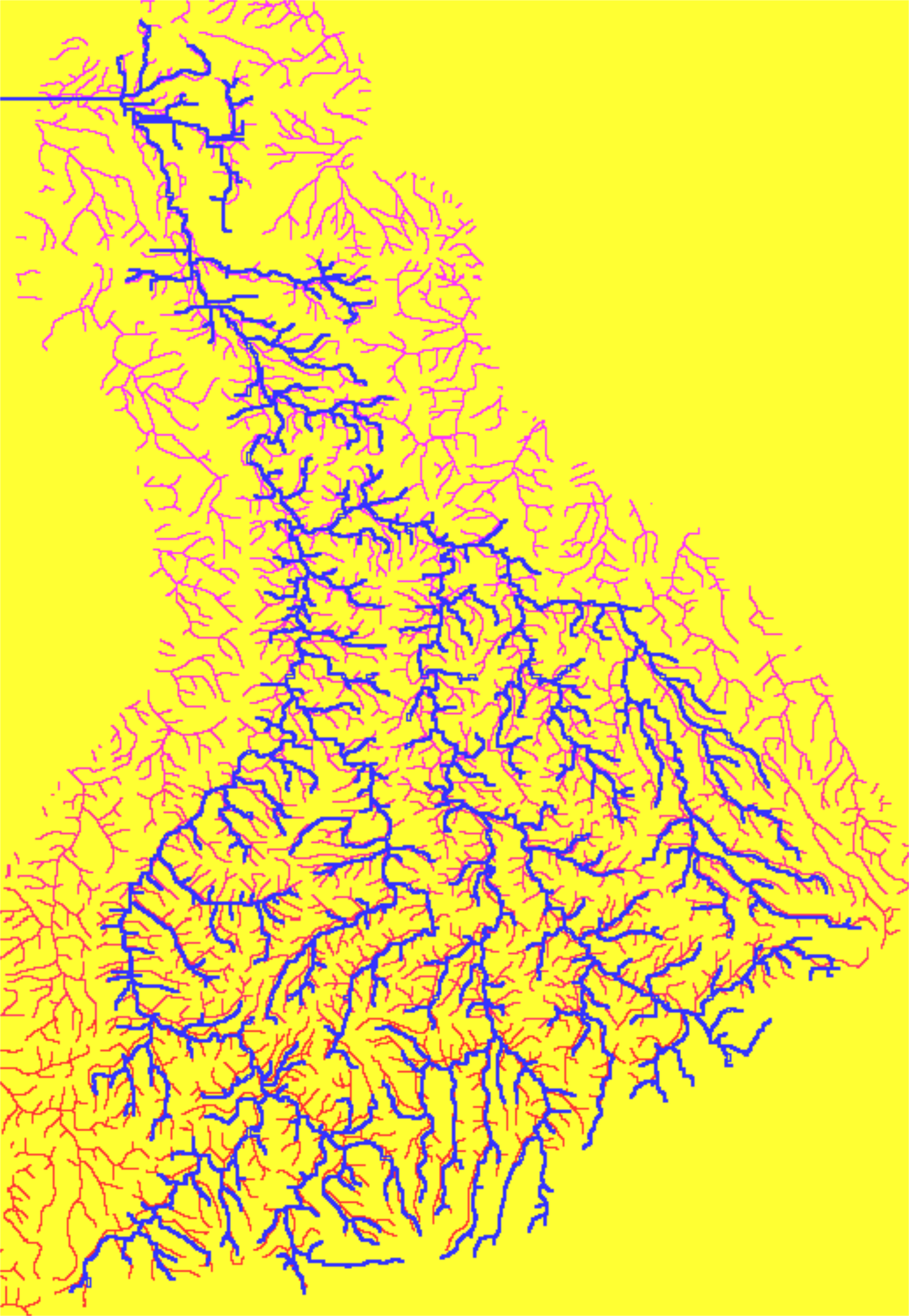
[fig:comparison_river_networks]
4.1.2 How to Choose Spatial Resolution?
Answering the first question, suggests using the so-called „thousand-million“ rule as a rough guide: take the area of the region under study and divide it by one million to give the appropriate cell size (area) to be used, then multiply the cell size chosen by one thousand which is then the minimum drainage area of watersheds that should be delineated from this DEM. This rule should not be understood as an absolute one, but should be treated with a certain level of approximation.
According to this rule, 930 m resolution should be used for delineation of a watershed with the drainage area of 4000 km2, 460 m resolution for a 1000 km2 watershed, 90 m for a 40 km2 watershed, and 30 m for a 5 km2 catchment. This is in agreement with our modelling experience from the studies performed in the Elbe drainage basin, where 100 m resolution was acceptable to represent a catchment of 64 km2, 200 m resolution was sufficient to delineate a watershed with an area of 535 km2, and 1000 m resolution was satisfactory for extracting watersheds with an area of 3,000-4,000 km2.
also provides a useful Table showing the recommended cell size of DEM for some typical applications. For example, for a region size of 1000 km2 a linear cell size of 30 m, and a sub-basin size of 5 km2 are recommended. In the region with an area of 8000 km2 the sub-basins of 40 km2 can be delineated based on 90 m resolution. For a region size of 200,000 km2 the recommended resolution is 460 m, and the sub-basin size 4000 km2.
Following this rule more strictly, we can suggest the following for some commonly used resolutions:
| Linear cell size, m | Cell area, km2 | Sub-basin area, km2 | Region or basin size, km2 |
|---|---|---|---|
| 30 | 0.0009 | 1 | 1,000 |
| 100 | 0.01 | 10 | 10,000 |
| 200 | 0.04 | 40 | 40,000 |
| 500 | 0.25 | 250 | 250,000 |
| 1000 | 1. | 1,000 | 1,000,000 |
Of course, in practice these recommendations should be used with some degree of freedom.
4.1.3 How to Choose the Average Sub-basin Area?
The second question relates to the upper limit of the sub-basin area, below which the effect of the river network can be neglected, and the choice of the average sub-basin area when creating the sub-basin map.
According to , the effect of the channel network becomes important for basins larger than about 10 km2, where the time constant of the network (i.e. travel time through it) becomes as long as for the infiltration phase. This is especially important for lowland, where the time constant may be very large.
On the other hand, in mountainous areas, where the time constant is rather low, the sub-basin area must be restricted due to climate gradients, because, as it was already explained in Chap. 1, the climate input in SWIM is considered to be homogeneous in sub-basins.
It is also known that 5 to 10 km (or 25 to 100 km2) appears to be the minimum scale, above which inhomogeneities in land surface properties can trigger specific mesoscale atmospheric circulation systems, which have a definite impact on interactions between land surface and the atmosphere .
So the following pragmatic conclusion might be drawn: an average sub-basin area, where the effect of the river network may be neglected, should be in a range of 10 to 100 km2 and definitely not larger than 100 km2.
The restrictions on average sub-basin area and time step influence the computing time, and, taken together with the data availability, define the upper limit of the sub-basin area for the model application. An adequate spatial disaggregation should allow the applicability of the model to be extended to larger basins.
4.1.4 GRASS GIS Overview
GRASS (Geographic Resource Analysis Support System) is a public domain raster GIS originally developed by the Environmental Division of the US Army Construction Engineering Research Laboratory (USA-CERL) as a general-purpose spatial modelling and analysis package. Since then, GRASS has evolved into a powerful tool with a wide range of applications in many different areas of scientific research. The new headquarters for GRASS support, research, and development is at Baylor University, the Department of Geology. Recently GRASS was upgraded to version 4.2, and the version 5.0 is underway.
GRASS is highly interactive and graphically oriented, providing tools for developing, analysing, and displaying spatial information. GRASS runs through the use of standardised command line input or under the X Window system under the UNIX environment. The following data formats are supported by GRASS:
raster,
vector,
sites,
satellite and air-photo image,
import from ASCII, DXF, Image, and others,
export to ASCII, DXF, Image, and others.
Though GRASS is the raster-based GIS, it can handle different data representations:
raster (or grid cell) data can be analysed, overlayed, recalculated,
vector data can be combined with raster data for display or analysis,
point data can be used to represent the locations of significant sites.
New maps can be digitised or scanned. Maps can also be transferred from other GIS systems like ARC/INFO. Data files can be developed for large or small geographic regions at any scale desired within the limits of the source data and the storage capacity of the hardware.
GRASS was successfully coupled with a number of hydrological and water quality models, like ANSWERS, AGNPS, TOPMODEL, SWAT, and SWIM (Srinivasan and Engel, 1991; Rewerts and Engel, 1991; Chairat and Delleur, 1993; Srinivasan and Arnold, 1994; Krysanova et al., 1998a) in order to facilitate input of spatially-distributed information and enhance the use and utility of the models.
First of all, GRASS raster capabilities are very attractive for the use in spatially-distributed hydrological modelling, because spatial data can be easily translated from the GIS to the model in order to initialise it, and the model outputs can be transferred to GIS again for visualisation and analysis purposes. Second, GRASS is a public domain GIS, all program codes are available. This is different from other packages like ARC/INFO, and significantly facilitates further software development. Third, GRASS is written in the C programming language, which is also widely used for modelling. Forth, GRASS is flexible enough for a variety of applications, as soon as data layers can be transported to and from several other GIS, including ARC/INFO. Last, but not least, GRASS has specific programs for hydrological modelling and interpolation, which can be very useful.
According to our experience the combination of ARC/INFO and GRASS packages can be especially powerful, when ARC/INFO is used mainly for preparation and editing of basic map layers, and afterwards GRASS is used for analysis, reclassification, overlaying, recalculation and application of specific hydrological tools.
4.1.5 Useful GRASS Programs and Functions
GRASS includes special programs and functions for Display (starting with d. ), General functions (g. ), Raster functions (r. ), Vector functions (v. ), Sites functions (s. ), Imagery functions (i. ), as well as some other contributed programs and shell scripts.
Import/Export programs There are a number of transformation programs between GRASS and different other formats: ASCII (v.in.ascii, v.out.ascii, r.in.ascii, r.out.ascii), ARC/INFO (v.in.arc, v.out.arc, r.in.ascii, r.out.ascii), DXF (v.in.dxf, v.out.dxf), DLG (v.import), DLG-3 (v.in.dlg, v.out.dlg), MOSS (v.out.moss). When a map layer has been converted to a GRASS raster format, all raster support files (cellhd, cell_misc, cats, colr, and hist) must be checked for accuracy and completeness. The r.support program must be run to modify these files if necessary. Transformation routines sometimes do not work smoothly. It can be due to the fact that the requirements and steps are not sufficiently described in the Manual.
Conversion programs A GRASS database can be based upon one of four different coordinate systems: UTM, SPCS (State Plane Coordinate System), latitude/longitude, or Cartesian coordinate (x/y) system. The map projection that is most commonly used for maps in a GRASS database is the Transverse Mercator projection which is the basis for the to Universal Transverse Mercator (UTM) coordinate system. There are five programs available for conversion purposes:
m.ll2u - converts geographic coordinates to Universal Transverse Mercator (UTM) coordinates for a number of spheroids,
m.u2ll and m.region.ll - convert Universal Transverse Mercator (UTM) coordinates falling within the current geographic region to geographic (latitude/longitude) coordinates,
m.gc2ll - converts geocentric to geographic coordinates for a number of possible spheroids,
m.ll2gc - converts geographic coordinates to geocentric.
The use of geographic coordinates in GRASS is still rather restricted.
Display and printout It is not so easy to create the good-quality printed maps in GRASS that look professional. There is no automatic way to create legend with user-specified options, bar scale, north arrow. The p.map script file has to be created in advance in order to create a postscript file and then a map can be printed. The other possibility is to use any screendump or grab procedure, which is available in a number of packages, and then to add additional features using these tools. Some new capabilities in the map printing program are designed now.
Special hydrological support programs There are several programs in GRASS, which provide support for hydrological modelling. The program r.watershed is the main tool for delineation of basin and sub-basin boundaries based on DEM, and for calculating the LS (slope length and steepness) and S (slope steepness) factors of the Revised Universal Soil Loss Equation (RUSLE) (see more detailed description in ). There are some more hydrologically-oriented programs in GRASS, like r.basins.fill, r.cost, r.drain as well as the useful interpolation tools.
The r.basins.fill program is similar to r.watershed but does not require DEM. It generates a raster map layer depicting sub-basins, based on two maps: 1) the coded stream network (each channel segment is „coded“ with a unique category value) and 2) the ridges within the given watershed (including the ridge which defines the perimeter of the watershed). The resulting output raster map layer codes the sub-basins with category values matching those of the channel segments passing through them.
The r.cost program determines the cumulative cost of moving to each cell on a cost surface (the input raster map) from other specified cell(s) whose locations are specified by their coordinates, and the r.drain program traces a flow through a least-cost path in an elevation model. The results for cells are similar to those obtained when using the seg version of the r.watershed program.
Interpolation programs There are two programs in GRASS for the interpolation from point data (s.surf.idw and s.surf.tps) and two programs for the interpolation from raster data (r.surf.idw and r.surf.idw2). The s.surf.idw fills a raster matrix with interpolated values generated from a set of irregularly spaced data points using numerical approximation (weighted averaging) techniques. The interpolated value of a cell is determined by values of nearby data points and the distance of the cell from those input points. In comparison with other methods, numerical approximation allows representation of more complex surfaces (particularly those with anomalous features), and restricts the spatial influence of any errors.
The s.surf.tps interpolates and computes topographic analysis from given site data (digitised contours, climatic stations, drill holes, etc.) to GRASS raster format using spline with tension. As an option, simultaneously with interpolation, topographic parameters like slope, aspect, profile curvature (measured in the direction of the steepest slope), tangential curvature (measured in the direction of a tangent to a contour line) or mean curvature are computed and saved as raster files. Topographic parameters are computed directly from the interpolation functions so that the important relationships between these parameters are preserved. The equations and their interpretation are described in .
Two programs r.surf.idw and r.surf.idw2 fill a grid cell (raster) matrix with interpolated values generated from a set of input layer data points or irregularly spaced data points. They use a numerical approximation technique based on distance squared weighting of the values of nearest data points. The number of nearest data points used to determine the interpolated value of a cell can be specified by the user (default: 12 nearest data points). Unlike r.surf.idw2, which processes all input data points in each interpolation cycle, r.surf.idw attempts to minimise the number of input data for which distances have to be calculated. Execution speed is therefore a function of the search effort and does not increase appreciably with the number of input data points. The r.surf.idw2 does not work with latitude/longitude data, in such a case the r.surf.idw should be used.
There are a number of useful GRASS commands, which are necessary for any SWIM user. They are needed for visualisation, recalculation, and reclassification of map layers. In the Appendix I the most useful GRASS commands are listed, which are needed for spatial data preparation.
4.1.6 Map Export from ARC/INFO to ASCII Format
Raster Data in ARC/INFO A raster data set in ARC/INFO is called a "Grid". All operations on grids are performed in the module with the same name. The resolution (or cell size) of any existing grid can be changed using the resample function, which offers different algorithms for categorial and continuous data. Conversion from vector to raster data in ARC/INFO can be either done on the Arc prompt, or within Grid. Both procedures are similar and can be performed with polygon, line or point input data. The user has to define the desired cell size, because one coverage can be gridded using different resolutions. By defining the coordinates of a lower left corner and a desired number of rows and columns, the processing can be focussed on a certain part of the coverage, if necessary. As GRASS version 4.2 does not yet support the NODATA data format, it is recommended to select ARC/INFO’s ZERO option using "0" as NODATA (or background) value.
Data Exchange between ARC/INFO and GRASS As neither GRASS 4.2 can import ARC/INFO grids, nor ARC/INFO can read GRASS raster maps directly, the data exchange between both systems should be performed using ASCII format. Both systems can produce and read ASCII files containing the data as a continuous stream of values separated by blanks. The information about how to produce a raster map for the system is stored in a header section containing the coordinates of the corner (or north, south, east west coordinates) and the number of rows and columns. ARC/INFO’s header format looks like
NCOLS xxx NROWS xxx XLLCORNER xxx YLLCORNER xxx CELLSIZE xxx NODATA_VALUE xxx,
whereas GRASS uses the following header:
north: xxx south: xxx east: xxx west: xxx rows: xxx cols: xxx
An example of data conversion Let us assume that we want to grid a polygon coverage called "lupoly" containing land use information (item lu-code) with cell size 50 and a line coverage "fgw" containing the stream network of the same region. The necessary commands are listed below (the comments are between **).
Step 1: Usage: POLYGRID <in_cover> <out_grid> value_item lookup_table weight_table Arc: POLYGRID lupoly lugrd lu-code
Converting polygons from lupoly to grid lugrd Cell Size (square cell): 50 Convert the Entire Coverage? (Y/N): y Number of Rows = 648 ** the value is calculated by the program** Number of Columns = 604 ** the value is calculated by the program**
Step 2: Usage: LINEGRID <in_cover> <out_grid> value_item lookup_table weight_table Arc: LINEGRID fgw fgwgrd
Converting arcs from fgw to grid fgwgrd Cell Size (square cell): 50 Convert the Entire Coverage(Y/N)?: y Enter background value (NODATA | ZERO): zero Number of Rows = 493 ** the value is calculated by the program** Number of Columns = 553 ** the value is calculated by the program**
An example of changing the cellsize of an existing grid Let us assume that we want to change the cell size of lugrd from its original size of 50 cells to 100 cells using the nearest-neighbour assignment as default option. (N.B.: This of course could be done earlier when prompted during POLYGRID).
Arc: grid ** starts the grid module**
Grid: lugrd2 = resample(lugrd,100) Resample ... Grid: quit ** leaves the grid module**
An example of export to ASCII file Let us assume that now we want to export lugrd and fgwgrd to ASCII files.
Usage: GRIDASCII <in_grid> <out_ascii_file> item Arc: GRIDASCII lugrd lugrd.txt Arc: GRIDASCII fgwgrd fgwgrd.txt
The header of lugrd.txt is: ncols 604 nrows 648 xllcorner 4492676.68 yllcorner 5884875.398 cellsize 50 NODATA_value -9999
The header of fgwgrd.txt is: ncols 553 nrows 493 xllcorner 4494452.5 yllcorner 5886652 cellsize 50 NODATA_value -9999
It is obvious that although both grids have the same cell size, they do not match, because their llcorners’ coordinates’ difference is not a multiple of their cell size. In such a case it is recommended to use the coordinates of lugrd as an input to LINEGRID as shown in the following example.
An example of producing matching grids The following commands should be done:
Usage: DESCRIBE <geo_dataset> Arc: DESCRIBE lugrd
Description of Grid LUGRD Cell Size = 50.000 Data Type: Integer Number of Rows = 648 Number of Values = 14 Number of Columns = 604 Attribute Data (bytes) = 8
BOUNDARY STATISTICS Xmin = 4492676.680 Minimum Value = 111.000 Xmax = 4522876.680 Maximum Value = 512.000 Ymin = 5884875.398 Mean = 225.421 Ymax = 5917275.398 Standard Deviation = 42.130
Arc: LINEGRID fgw fgwgrd Converting arcs from fgw to grid fgwgrd Cell Size (square cell): 50 Convert the Entire Coverage(Y/N)?: n **in Example 1 we entered y ** Grid Origin (x, y): 4492676.680,5884875.398 **values taken from lugrd ** Grid Size (nrows, ncolumns): 648,604 **values taken from lugrd **
Enter background value (NODATA | ZERO): zero Number of Rows = 648 Number of Columns = 604 Arc: GRIDASCII fgwgrd fgwgrd.txt
Now fgwgrd.txt’s header looks as follows: ncols 604 nrows 648 xllcorner 4492676.68 yllcorner 5884875.398 cellsize 50 NODATA_value -9999
After the header information has been changed, both ASCII files are almost ready to be imported to GRASS running r.in.ascii (after changing the header).
An example of changing the header information The map exported from ARC/INFO in ASCII format has the heading, which consists of six lines, describing coordinates of the lower left corner, number of columns and rows, and the cell size, e.g.:
ncols 349 nrows 542 xllcorner 69367.3 yllcorner 37980.7 cellsize 1000 NODATA_value -9999
However GRASS requires slightly different format for its r.in.ascii program, describing the coordinates of north, south, east and west, and the number of rows and columns, like:
north:579980.7 south: 37980.7 east: 418367.3 west: 69367.3 rows: 542 cols: 349
The ARC/INFO export file in ASCII format can be transformed to GRASS input ASCII format using the program arc2grass, which is included in the SWIM model package.
4.1.7 Watershed Analysis Program r.watershed
Delineation of watersheds from the Digital Elevation Model (DEM) is the first necessary step in many hydrological applications. A procedure that has become a standard one is based on the eight-direction basis in which each grid cell is connected to one of its eight neighbour cells according to the direction of steepest descent. Another possibility is to use the four-direction procedure for watershed delineation.
Based on an elevation grid, a grid of flow direction is built, and then a map of flow accumulation is derived from the flow direction map, counting the number of cells upstream of a given cell. Streams are identified as lines of cells whose flow accumulation exceeds a specified threshold number of cells and thus a specified upstream drainage area. This threshold number must be specified in advance. Watershed is delineated as the set of all cells draining through a given cell.
GRASS program r.watershed is the main tool for delineation of basin and sub-basin boundaries and calculating the LS (slope length and steepness) and S (slope steepness) factors of the Revised Universal Soil Loss Equation (RUSLE) in GRASS.
There are two versions of this program available in GRASS: ram and seg. Which of them is run depends on whether the -m flag is set or not. The ram version uses virtual memory managed by the operating system to store data and is much faster than the seg version. The seg version (with the -m flag) uses the memory on disk which allows larger maps to be processed but is considerably slower.
The seg version uses the AT least-cost search algorithm to determine the flow of water over the landscape and is more reliable than ram. In addition to the elevation map, maps of depressions in the landscape and blocking terrain can be provided to assure more reliable watershed boundaries.
Due to memory requirements of both seg and ram versions of the program, it is quite easy to run out of memory. If the resolution of the current region cannot be increased, more memory needs to be added to the computer. GRASS Reference Manual provides recommendations on how to use the coarser resolution. Masking out unimportant areas is another means to reduce processing time significantly if the watershed of interest occupies only a part of the overall area. According to our experience, the seg version of the program is much more reliable. Our recommendation is to use only this version for watershed delineation (using the -m flag).
After the watersheds are delineated for a certain region, an analysis of output maps has to be done in order to identify the basin under study and its sub-basins. For this purpose the basin, accumulation, and streams output maps are needed, as well as any available digitised maps of the basin boundaries or river network. Comparison of digitised and calculated rivers, digitised and calculated watershed boundaries can be very helpful in order to find some mistakes or inconsistencies in the DEM. An example of resulted sub-basin map with the river network is given in .
After correction of the DEM the procedure r.watershed can be repeated. It is also quite difficult to find an appropriate threshold value from the very beginning. Usually, it is necessary to repeat the procedure several times with different thresholds. The user has to remember that LS and S factors are multiplied by 100 for the GRASS output map layer, since they are usually small numbers.
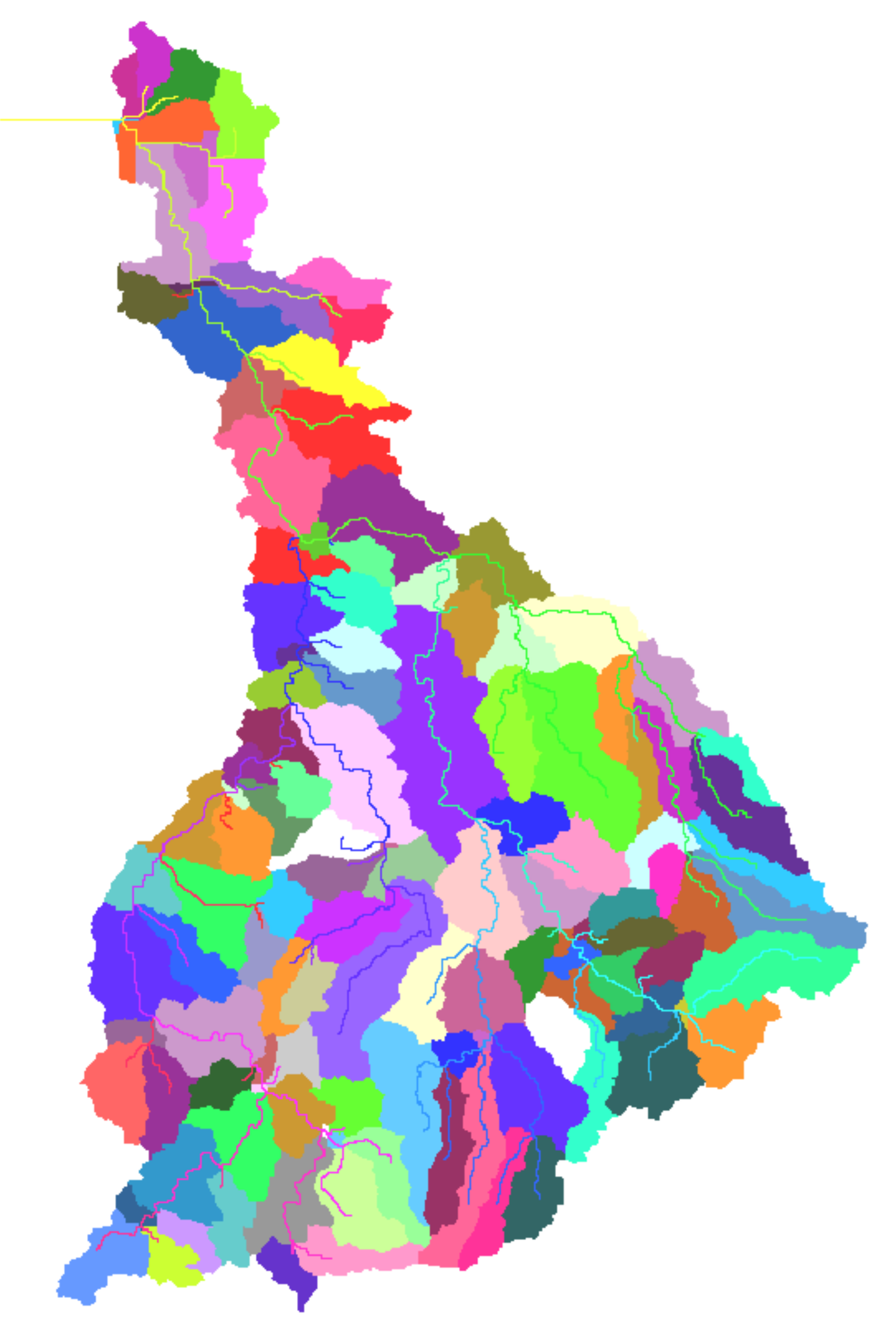
[fig:Virtual_subbasins_Mulde_river_basin]
4.1.8 DEMO Data Set
Here the DEMO data set for spatial data preparation is described. The maps for the Glonn basin in Bavaria (drainage area 392 km2) were used for that.
Input data in ASCII format The exemplary export files in ASCII format produced in ARC/INFO are located in the directory /grassdata. They are: the Digital Elevation Model map in the file glonn160-dem.asc, and the soil map in the file glonn160-soil.asc. The program arc2grass can be used for converting the ARC/INFO export files to GRASS format. The resulting ASCII files for these two and other maps, which are ready for GRASS import, are located in the same directory
| - glonn160-dem.txt | - DEM map, |
| - glonn160-lus.txt | - land use map, |
| - glonn160-soil.txt | - soil map, |
| - glonn160-fluss.txt | - a river map, |
| - glonn160-rivnet.txt | - a more detailed river map, |
| - glonn160-pegel.txt | - gage station map, |
| - glonn160-clst.txt | - climate stations map, |
| - glonn160-prst.txt | - precipitation stations map, |
| - glonn160-clst-this.txt | - a map with Thiessen polygons for climate stations, |
| - glonn160-prst-this.txt | - a map with Thiessen polygons for precipitation stations. |
Geographic location Let us assume that the geographic location with the name glonn160 is created by the user usern in the directory /usern/databases. Here 160 indicates the resolution of maps in this location (which was chosen in accordance with the resolution of available DEM map). The directory /usern/databases contains at least two subdirectories: /PERMANENT and /usern. The directory /PERMANENT describes the name (file MYNAME) and coordinates (file WIND) of the geographic location. In our case the file WIND looks as following:
| proj: | 0 |
| zone: | 0 |
| north: | 6098669 |
| south: | 6064429 |
| east: | 123951 |
| west: | 73871 |
| cols: | 313 |
| rows: | 214 |
| e-w resol: | 160 |
| n-s resol: | 160 |
The directory /usern/databases/glonn160/usern is designated for all GRASS files in this geographic location, which will be stored under subdirectories: cats, catts_dig, cell, cell_misc, cellhd, colr, dig, dig_ascii, dig_att, dig_cats, hist. Here the user name usern corresponds to the name of MAPSET, which is asked always when starting GRASS session. All files from this directory can be copied by any other user and used independently.
Map input to GRASS As a first step, a number of maps can be created by introducing data in ASCII format to GRASS using r.in.ascii command. For example, the following maps listed in can be introduced from available ASCII data:
| GRASS map | Map description | The corresponding source ASCII file |
|---|---|---|
| Table – Continued from previous page | ||
| GRASS map | Map description | The corresponding source ASCII file |
| dem | DEM | glonn160-dem.txt |
| lus | Land use | glonn160-lus.txt |
| soil | Soil | glonn160-soil.txt |
| fluss | River network | glonn160-fluss.txt |
| flussnet | Detailed river network | glonn160-rivnet.txt |
| pegel | Gage station | glonn160-pegel.txt |
| clst | Climate stations | glonn160-clst.txt |
| prst | Precipitation stations | glonn160-prst.txt |
| clstthis | Thiessen polygons for climate stations | glonn160-clst-this.txt |
| prstthis | Thiessen polygons for precipitation stations | glonn160-prst-this.txt |
Program r.watershed After that the program r.watershed can be applied to the Digital Elevation Model dem in order to create sub-basin maps. Let us assume that we applied this program six times (always with a flag –m) with different thresholds. The threshold is defined as a minimum size of the exterior watershed basin. As a result, a number of sub-basin maps (basN) and stream network maps (rivN) will be created as listed in :
| Threshold (number of cells) | Corresponding area, km2 | Created maps |
|---|---|---|
| Table – Continued from previous page | ||
| Threshold (number of cells) | Corresponding area, km2 | Created maps |
| 3600 | 92.16 | bas1, riv1 |
| 1800 | 46.08 | bas2, riv2 |
| 900 | 23.04 | bas3, riv3 |
| 200 | 5.12 | bas4, riv4 |
| 100 | 2.56 | bas5, riv5 |
| 50 | 1.26 | bas6, riv6 |
We can compare the average, minimum and maximum sub-basin area for three different sub-basin maps bas3, bas4, and bas6, created with different thresholds (see and ).
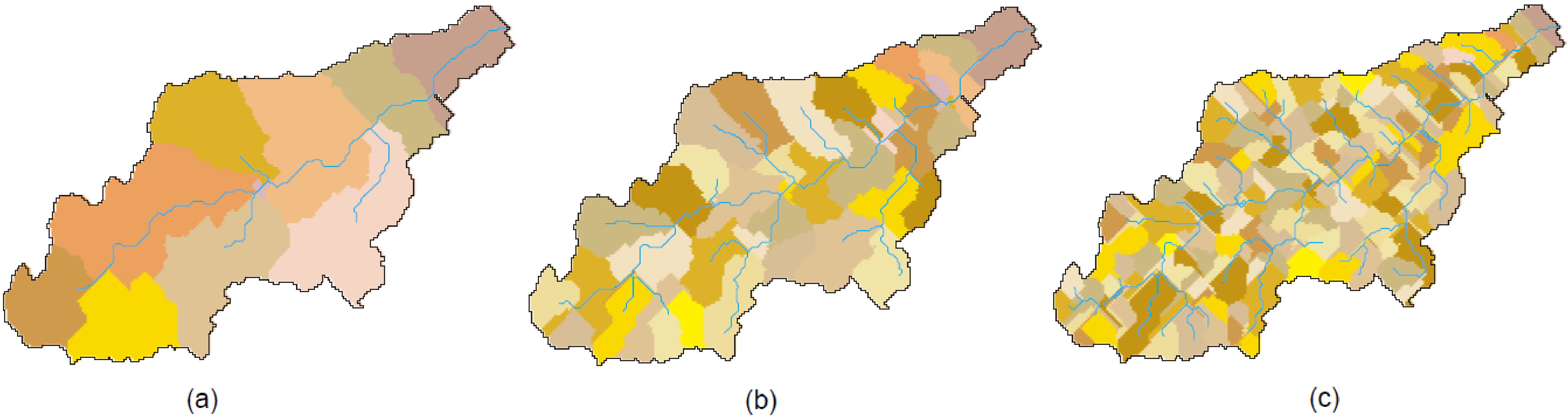
[fig:r_watershed_900_200_50]
| Raster map name) | Number of sub-basins | Average sub-basin area, km2 | Minimum sub-basin area, km2 | Maximum sub-basin area, km2 |
|---|---|---|---|---|
| Table – Continued from previous page | ||||
| Raster map name) | Number of sub-basins | Average sub-basin area, km2 | Minimum sub-basin area, km2 | Maximum sub-basin area, km2 |
| bas3 | 10 | 40.6 | 1.02 | 72.2 |
| bas4 | 42 | 9.7 | 0.36 | 19.1 |
| bas6 | 162 | 2.5 | 0.05 | 11.2 |
As we can see, 10 sub-basins with an average area of 40.6 km2 were created with threshold 900 cells, or 23.04 km2, 42 sub-basins with an average area of 9.7 km2 were created with threshold 200 cells, or 5.12 km2, and 162 sub-basins with an average area of 2.5 km2 were created with threshold 50 cells, or 1.26 km2. In other words, the threshold corresponds approximately to ½ of the average area of created sub-basins. This has to be taken into account when estimating the threshold values. Finally, the three sub-basin maps: bas36, bas44 and bas64 were chosen for model application.
Reclassification and analysis The original land use map lus has to be reclassified to SWIM land use categories. The latter one, as well as the dem and soil maps have to be clipped using a mask (e.g. corresponding to the bas3 map), to get the final maps dem3, lus3, soil3, which can be used by Interface. Finally, the four maps (e.g. dem3, lus3, soil3 and bas3) are ready for SWIM/GRASS interface.
The programs r.stats and r.report (see Appendix I) are useful for the analysis of obtained maps. For example, using the function r.report as
r.report -z map=soil3 units=k,p output=gl160-soil.rep
we can get the following report about the soil map soil, indicating areal distribution of soil categories (in km2 and in percent). For example, Tab. 4.5 includes GRASS report about the soil map soil3, indicating areal distribution of soil types.
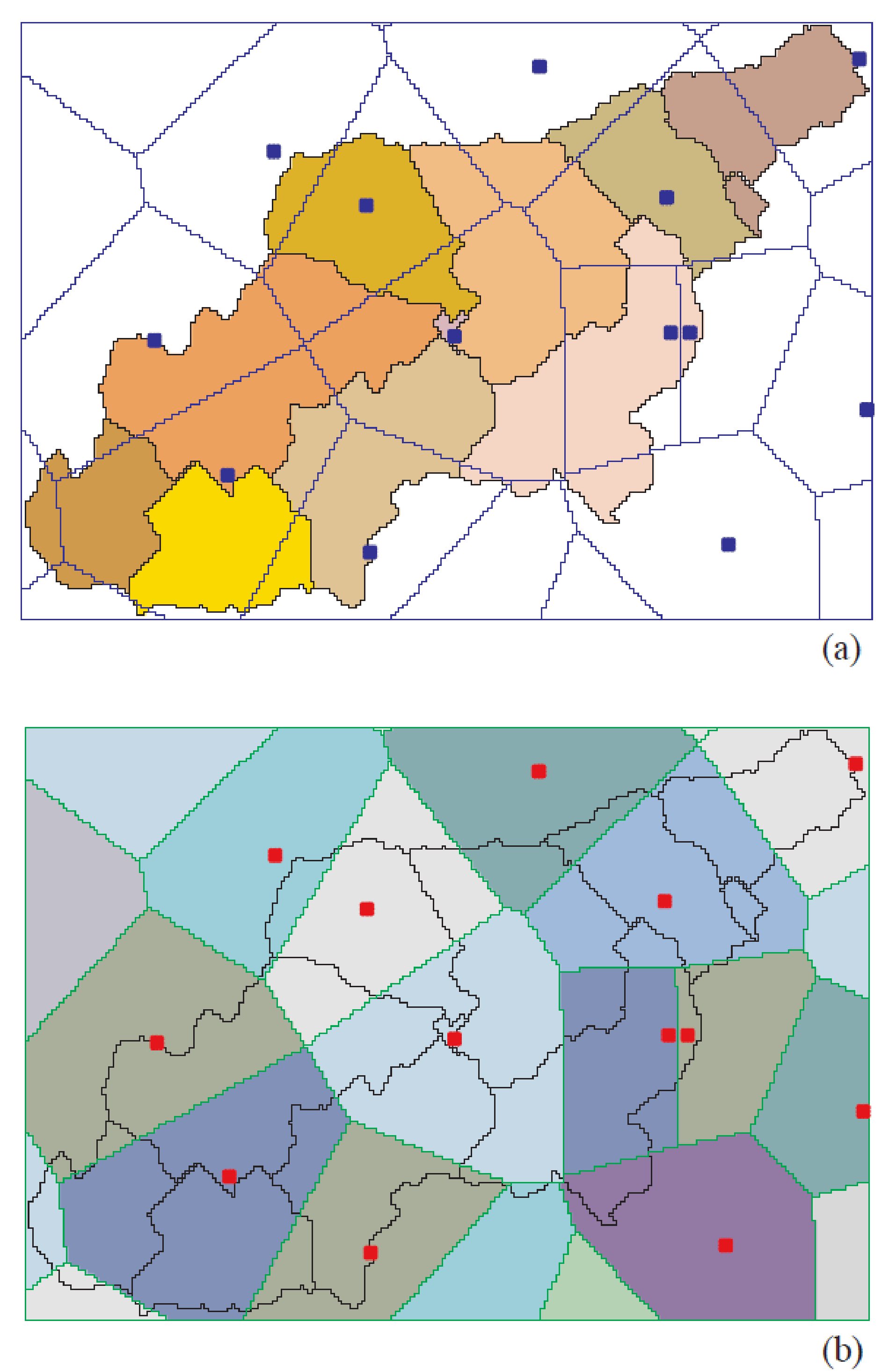
[fig:prec_station_thiessen_maps]
demonstrates an overlay of sub-basins (bas3), precipitation stations (prst2), and Thiessen polygons for precipitation stations. The report about two of these maps:
r.report -z map=bas3,prstthis units=k,p output=glonn-bas36-prstthis.rep
is given in . Such a report can be very helpful in establishing the connection between sub-basins and precipitation stations (weighting coefficients).
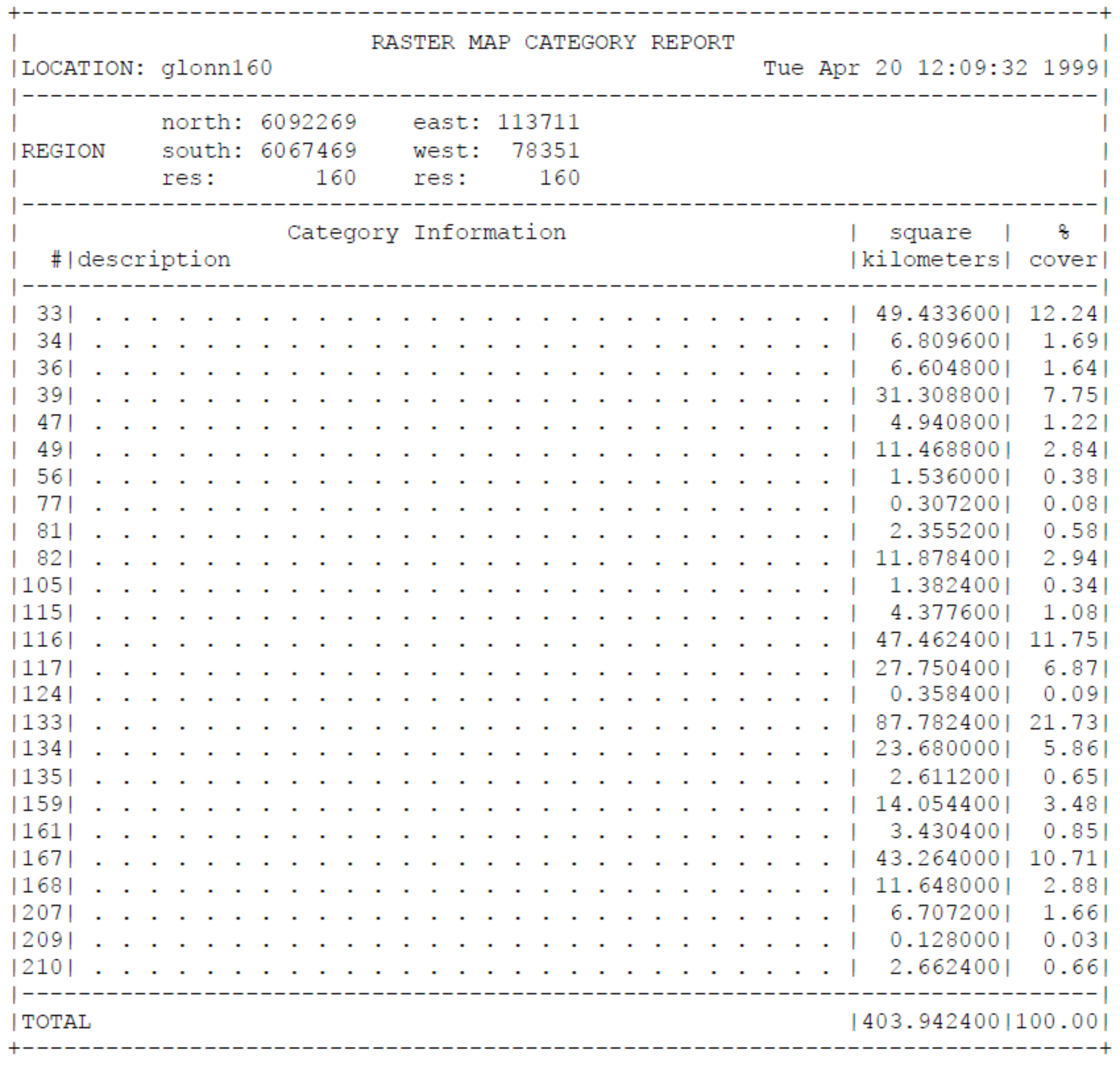
[fig:GRASS_report_soil_map_soil3]
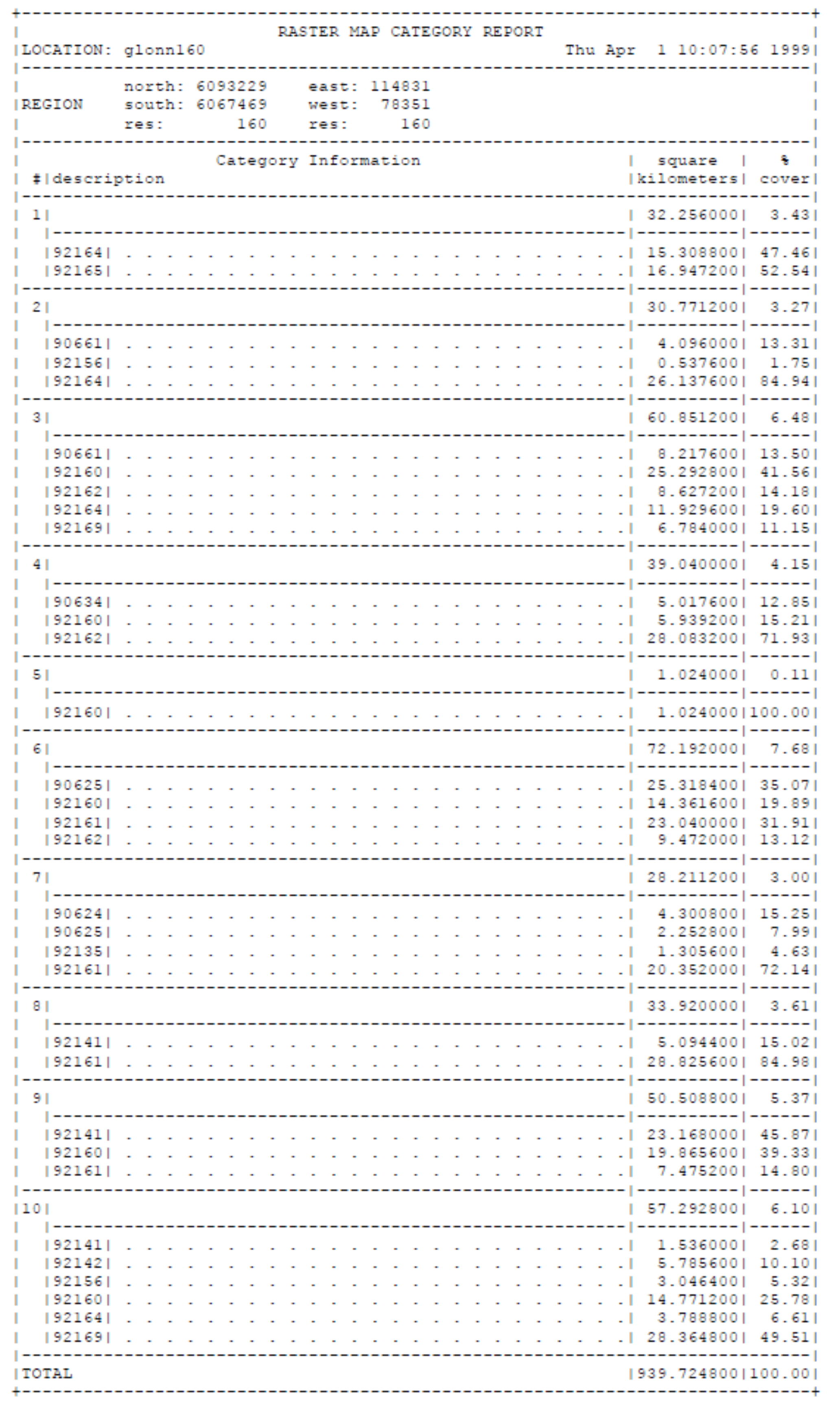
[fig:GRASS_report_sub-basin_map_bas3]
4.2 SWIM/GRASS Interface
Throughout SWIM/GRASS, two primary types of interface input are used:
Text input that can be completed by hitting the RETURN key. In most cases, if no text was entered, the given question or operation is cancelled. Most often the text input will consist of the name of a new or existing map or project name, in which case entering the word "list" will provide a list of currently used names.
Text or menu options that can be completed by hitting the ESC (escape) key. This type of interface is used for menus or for entering tables of parameters. All menus have a default answer of Exit (0), so that by simply hitting ESC one may leave the program’s menus.
The following provides a keystroke guide, which is helpful when using the parameter entry worksheets that use this interface:
| key | the function |
|---|---|
| <RETURN> | moves the cursor to next prompt field |
| <CTRL-K> | moves the cursor to previous prompt field |
| <CTRL-H> | moves the cursor backward non-destructively within the field |
| <CTRL-L> | moves the cursor forward non-destructively within the field |
| <CTRL-A> | copies the screen to a file named "visual_ask" in the users home directory |
| <CTRL-C> | where indicated (on the bottom line of the screen) can be used to cancel operation |
Starting GRASS and SWIM_INPUT Before running SWIM/GRASS interface, GRASS has to be started. For that, the user has to start GRASS:
grass4.2.1
The following information window will appear:
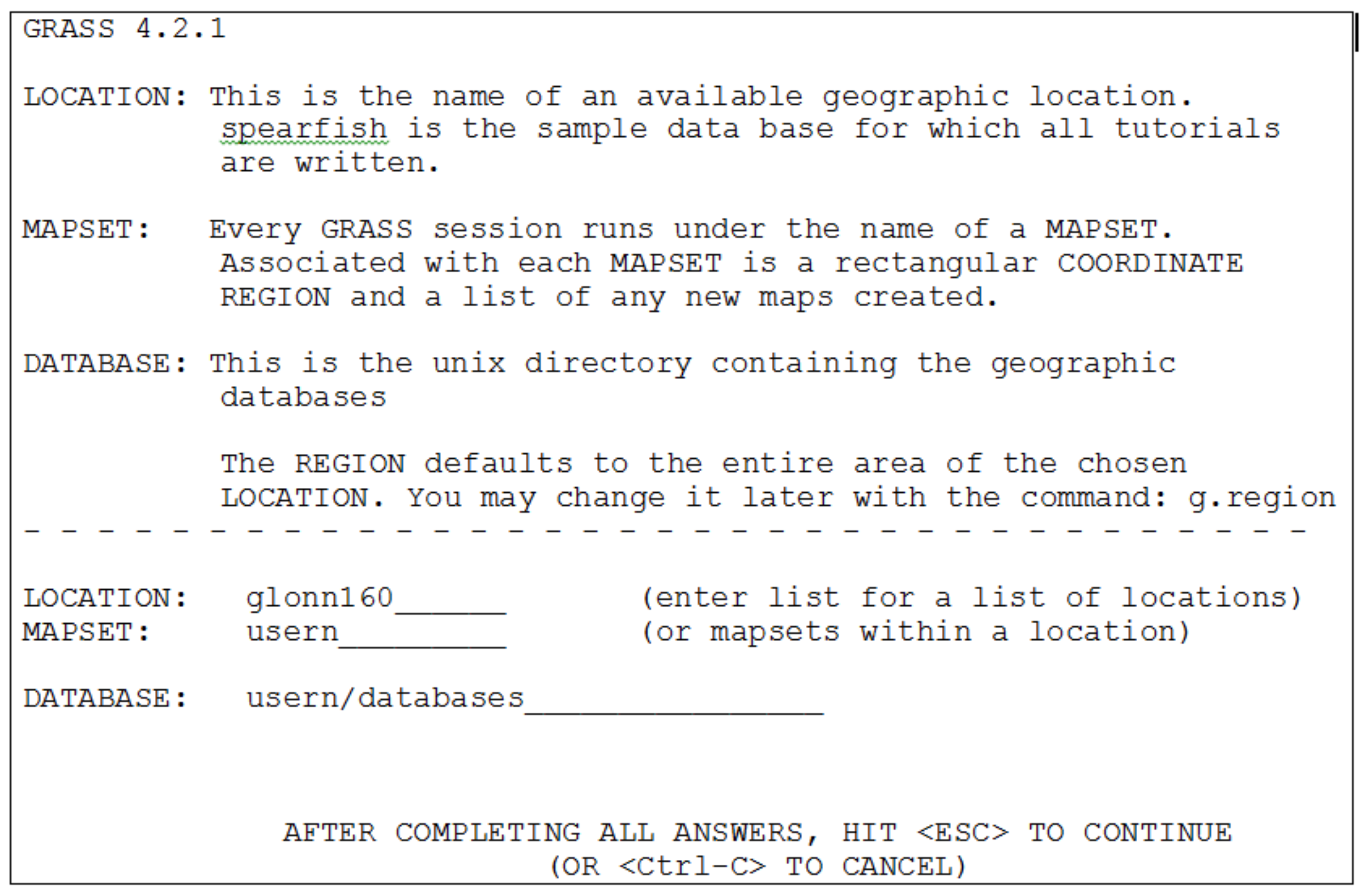
The Location and Database names are the last entered. If you need another ones, please change the names. After entering GRASS, the user can open the monitor with the command d.mon. After that SWIM/GRASS interface can be started:
cd usern/swiminput swim_input
The following window will appear:
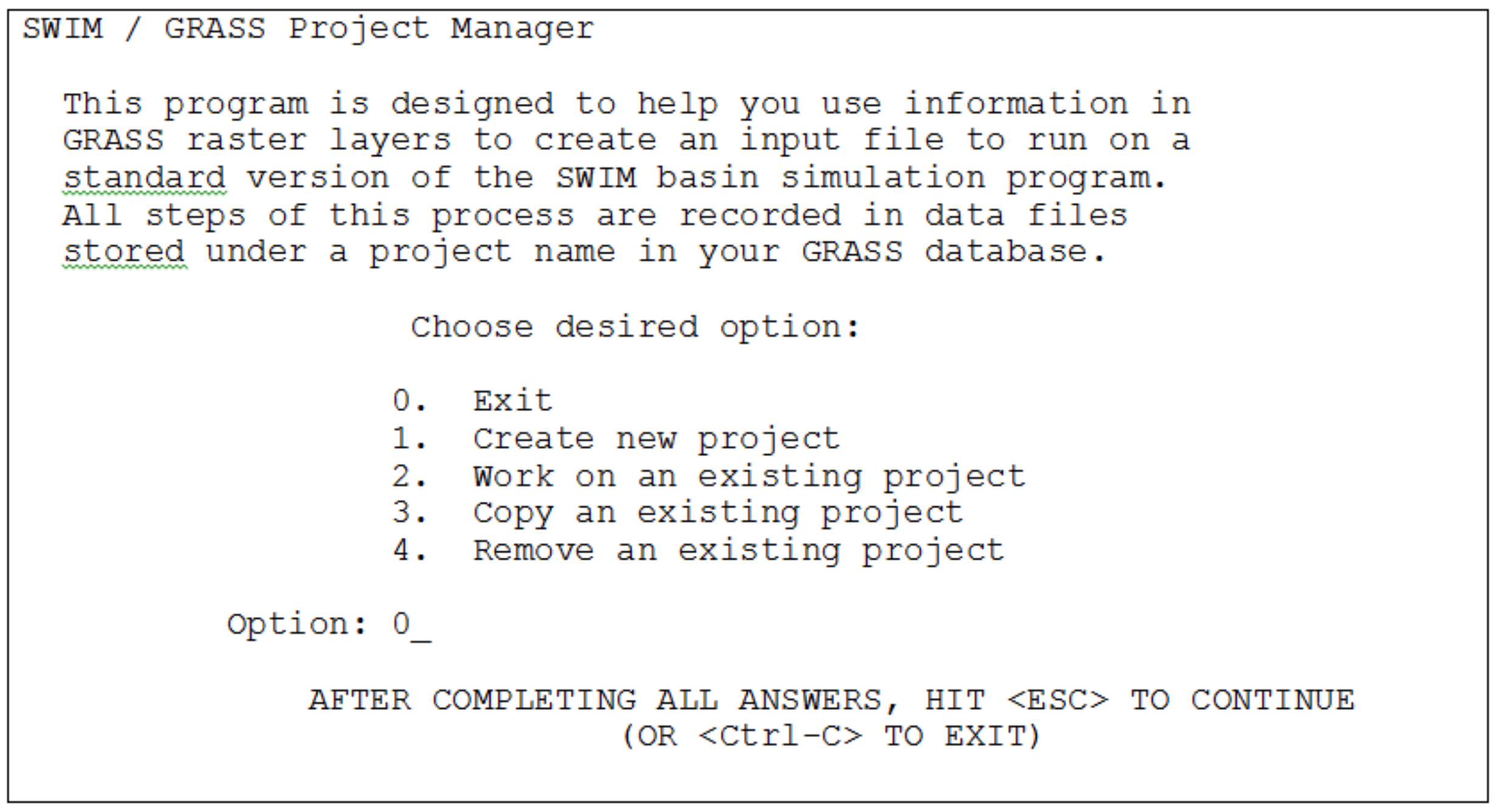
[fig:GRASS_project_manager]
Options of the main menu The user can use option 1 to create a new project, or option 2 to continue working on an existing project. If you want to create a new project, choose the option 1. After that you have to enter the project name. The name should correspond to the basin name, but it has to be not too long (maximum 8 letters), for example, we choose ‚gl‘:
Enter project name:
Enter ’list’ for a list of existing SWIM / GRASS project files Hit RETURN to cancel request > gl
Then the following Data Extraction Menu will appear:
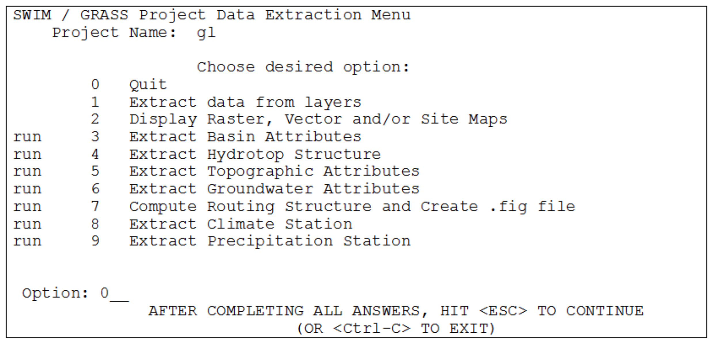
[fig:GRASS_Data_Extraction_Menu ]
Data Extraction Steps 3 to 7 have to be run one after another, after that option 0 has to be chosen. Steps 8 and 9 are not up to date, they have to be modified.
When the option 3 is chosen to extract basin attributes, the name of the basin and sub-basin map is asked. Assuming that we use the maps described in the previous section, the name ‚bas36‘ has to be entered:
Basin and Subbasin Map Enter ’list’ for a list of existing raster files Enter ’list -f’ for a list with titles Hit RETURN to cancel request > bas36
When the option 4 is chosen to extract the hydrotope structure, the names of three maps: 1) basin and sub-basin, 2) land use and 3) soil are asked:
Basin and Subbasin Map Enter ’list’ for a list of existing raster files Enter ’list -f’ for a list with titles Hit RETURN to cancel request > bas36 <bas36>
Landuse Map Enter ’list’ for a list of existing raster files Enter ’list -f’ for a list with titles Hit RETURN to cancel request > lus36 <lus36>
Soil Map Enter ’list’ for a list of existing raster files Enter ’list -f’ for a list with titles Hit RETURN to cancel request > soil36
When the option 5 is chosen to extract topographic attributes, the name of the elevation map has to be entered:
Elevation Map Enter ’list’ for a list of existing raster files Enter ’list -f’ for a list with titles Hit RETURN to cancel request > dem36
When the option 6 is chosen to extract groundwater attributes, the name of the groundwater alpha map is asked. If the user does not have such a map, an option ‚n‘ has to chosen:
Do you have groundwater alpha parameter map?(y/n) [y] n
The next step is to choose 7 in order to compute routing structure of the basin. If the routing structure is calculated without problems, the user gets a message about the outlet sub-basin, like:
outlet subbasin number is 1
Please note that the outlet sub-basin has to numbered with 1, otherwise the user has to recode the output. After that the user has to choose ‚0‘ to quit the SWIM/GRASS interface. The results will be stored in the directory:
in usern/databases/glonn160/usern/swim/gl,
which corresponds to the DATABASE/LOCATION/MAPSET/swim/projectname. In our case the full list of resulting files is the following:
,where the number n corresponds to the sub-basin number n+1.
Possible problem In some cases, option 7 runs not so smoothly, and the message like
Start checking the aspect through each subbasin More than one outlet from subbasins 1 and 40 More than one outlet found from subbasins 40 1 Do you agree with this?(y/n) [y]
can appear. If the user chooses ‚y‘, the routing structure file will be created, but without sub-basin 40. In such a situation ‚n‘ has to be chosen in order to edit aspect. After choosing ‚n‘, the programs asks:
Would you like to continue?(y/n) [y]
When the user answers: ‚y‘, the following Sub-basin Aspect Editing menu will appear:
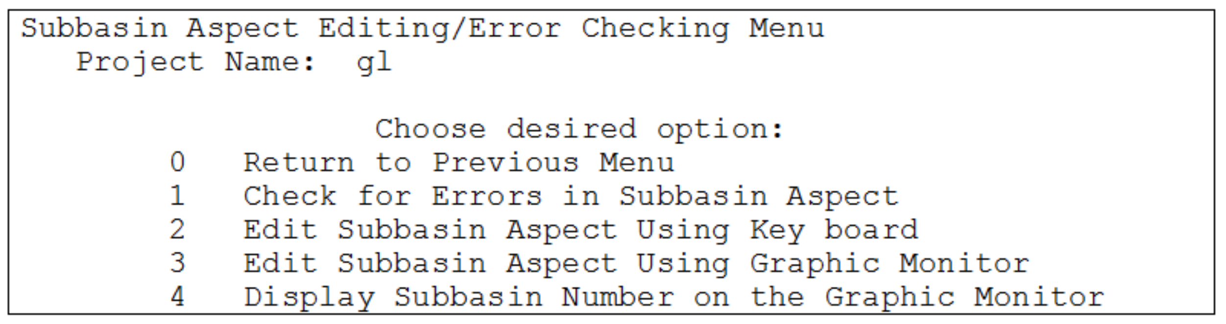
Please choose the option 3, and point on two sub-basins sequentially. For example, if you know that stream in sub-basin 40 flows to sub-basin 38, then point two sub-basins: first sub-basin 40, then sub-basin 38. After that click on non-basin area to finish.
Working on existing project If the user wants to continue working on an existing project, he/she can start from that point, where the project was stopped the former time.
4.3 Relational Data Preparation
4.3.1 An Overview of Relational Data
The full list of necessary relational data is the following:
Climate data: average, minimum and maximum daily air temperature, daily precipitation, and daily solar radiation,
soil geophysical and geochemical parameters,
crop types, crop rotation and crop management,
river discharge at the basin outlet,
water quality parameters (N, P, suspended solids) at the basin outlet,
river cross-sections or mean river width and depth,
rainfall intensity parameters.
The climate and soil data (1-4) are absolutely necessary to run the model.
Information about crop types in the basin, crop rotation and crop management (dates of planting and harvesting, dates and rates of fertilization) (5) is needed to initialise the model. If detailed information about crop management is not available for the studied basin, at least expert knowledge should be used in this case.
Measured river discharge and water quality parameters (6-7) are necessary for model validation.
River cross-sections (8) or mean river width and depth in several points of a basin (approximately one per sub-basin) can facilitate the model verification, especially for lateral processes (water and chemicals routing). The other way is to use the default stream width and depth parameters extracted from DEM by SWIM/GRASS interface.
Rainfall intensity parameters (9), which include
ten years frequency of I30 - the maximum annual half-an-hour rainfall,
ten years frequency of I360 - the maximum annual six-hours rainfall, and
long-term monthly maximum of the half-an-hour rainfall,
are necessary for erosion modelling.
In the following sections specific data requirements for climate, soil, crops, curve numbers are considered with some more detail.
4.3.2 Climate Data
The climate parameters necessary to drive the model are daily precipitation, air temperature (maximum, average, and minimum), and solar radiation. Usually, the climate data must be taken from meteorological and precipitation stations. This is absolutely necessary in the case of model validation for a specific basin. Note that the climate data have to be corrected, no missing values in form of –999 are allowed.
Usually, climate input is considered to be homogeneous at the level of sub-basins. The precipitation data has to be provided for as many stations as possible (approximately 1 station per 100 km2 area), while this is less important for the air temperature and solar radiation parameters.
According to our experience, the best is to use data from all available climate stations (parameters 1-3), located inside and close to the basin, in a combination with precipitation data from all available precipitation stations, also located inside the basin and close to it.
The following , and demonstrate the format of temperature, precipitation, and radiation data for SWIM. The other possibility is to put all climate data in one file, if the number of stations is not too large.
| Table – Continued from previous page | |||||
|---|---|---|---|---|---|
| YYYY | MON | DAY | 4116tmx | 4116tav | 4116tmn |
| 1981 | 1 | 1 | 3.5 | 0.4 | -1.7 |
| 1981 | 1 | 2 | 1.0 | 0.5 | -1.3 |
| 1981 | 1 | 3 | 5.8 | 3.9 | 0.7 |
| 1981 | 1 | 4 | 4.0 | 1.4 | 0.4 |
| 1981 | 1 | 5 | 0.5 | -1.6 | -3.5 |
| 1981 | 1 | 6 | -1.3 | -3.0 | -3.6 |
| 1981 | 1 | 7 | -3.4 | -6.8 | -10.5 |
| 1981 | 1 | 8 | -5.8 | -15.5 | -21.4 |
| 1981 | 1 | 9 | -4.8 | -7.8 | -21.8 |
| 1981 | 1 | 10 | -0.2 | -2.8 | -6.6 |
| 1981 | 1 | 11 | -1.2 | -2.6 | -4.3 |
| 1981 | 1 | 12 | -2.0 | -3.9 | -4.6 |
| .... | .. | .. | ... | ... | ... |
| Table – Continued from previous page | ||||||||
|---|---|---|---|---|---|---|---|---|
| YYYY | MON | DAY | 90625 | 90661 | 92141 | 92160 | 92161 | 92162 |
| 1981 | 1 | 1 | 12.2 | 12.4 | 7.6 | 10.4 | 7.6 | 8.5 |
| 1981 | 1 | 2 | 7.7 | 8 | 4.2 | 8.5 | 4.2 | 9.1 |
| 1981 | 1 | 3 | 7.8 | 4.5 | 8.3 | 5.4 | 8.3 | 6.2 |
| 1981 | 1 | 4 | 8.8 | 6.6 | 6.8 | 7.1 | 6.8 | 8.8 |
| 1981 | 1 | 5 | 9 | 6 | 6.2 | 7.8 | 6.2 | 5.6 |
| 1981 | 1 | 6 | 3.2 | 3.3 | 2.4 | 3.4 | 2.4 | 3 |
| 1981 | 1 | 7 | 1.7 | 2.1 | 1.4 | 1.4 | 1.4 | 1.5 |
| 1981 | 1 | 8 | 0.6 | 0 | 0.3 | 0.4 | 0.3 | 0.3 |
| 1981 | 1 | 9 | 0 | 1.4 | 0.4 | 0 | 0.4 | 0.9 |
| 1981 | 1 | 10 | 1.2 | 1.4 | 0.4 | 0.2 | 0.4 | 0.9 |
| 1981 | 1 | 11 | 0 | 0 | 0 | 0 | 0 | 0 |
| 1981 | 1 | 12 | 0 | 0 | 0 | 0 | 0 | 0 |
| .... | .. | .. | ... | ... | ... | ... | ... | ... |
| Table – Continued from previous page | |||
|---|---|---|---|
| YYYY | MON | DAY | 4117rad |
| 1981 | 1 | 1 | 171.0 |
| 1981 | 1 | 2 | 173.0 |
| 1981 | 1 | 3 | 186.6 |
| 1981 | 1 | 4 | 178.0 |
| 1981 | 1 | 5 | 173.0 |
| 1981 | 1 | 6 | 174.0 |
| 1981 | 1 | 7 | 241.0 |
| 1981 | 1 | 8 | 485.8 |
| 1981 | 1 | 9 | 170.0 |
| 1981 | 1 | 10 | 183.0 |
| 1981 | 1 | 11 | 171.0 |
| 1981 | 1 | 1 | 479.0 |
| .... | .. | .. | ... |
Climate input in the model is not fully automatised at the moment. Therefore, the subroutine cliread() has to be recompiled for new applications to take into account specific climate input: number of climate and precipitation stations, and their ‘attachment’ to sub-basins with specific weighting coefficients. Later, this routine has to be rearranged to allow fully automatised climate data input.
The other way is to use weather generator instead of actual climate parameters. The weather generator is attached to the model and can be initialised using monthly statistical data for the station(s) (see, e.g., ):
average monthly maximum temperature (e.g., line 3 in ),
average monthly minimum temperature (line 4),
coefficient of variation for monthly temperature (line 5),
average monthly solar radiation (line 6),
monthly maximum 0.5 hour rain for period of record (line 7),
monthly probability of wet day after dry (line 8),
monthly probability of wet day after wet (line 9),
monthly days with precipitation in a month (line 10) (can be used instead of monthly probabilities),
monthly mean event rainfall (line 11),
monthly standard deviation of rainfall (line 12),
monthly skew coefficient of daily rainfall (line 13).
| Table – Continued from previous page | ||||||||||||||
|---|---|---|---|---|---|---|---|---|---|---|---|---|---|---|
| 1.80 | 3.00 | 8.10 | 13.40 | 19.10 | 22.10 | 23.70 | 23.00 | 19.30 | 13.30 | 6.70 | 2.90 | |||
| -3.30 | -2.90 | -0.20 | 3.40 | 7.90 | 11.20 | 13.20 | 12.70 | 9.60 | 5.50 | 1.30 | -1.70 | |||
| 0.18 | 0.14 | 0.11 | 0.10 | 0.09 | 0.08 | 0.07 | 0.07 | 0.08 | 0.10 | 0.13 | 0.15 | |||
| 56. | 104. | 213. | 267. | 512. | 471. | 417. | 351. | 282. | 152. | 74. | 42. | |||
| 7. | 7. | 9. | 9. | 10. | 10. | 10. | 10. | 9. | 9. | 7. | 7. | |||
| 0.37 | 0.34 | 0.35 | 0.33 | 0.32 | 0.29 | 0.35 | 0.41 | 0.51 | 0.55 | 0.56 | 0.38 | |||
| 0.69 | 0.67 | 0.69 | 0.64 | 0.64 | 0.61 | 0.65 | 0.70 | 0.72 | 0.78 | 0.79 | 0.45 | |||
| 0.00 | 0.00 | 0.00 | 0.00 | 0.00 | 0.00 | 0.00 | 0.00 | 0.00 | 0.00 | 0.00 | 0.00 | |||
| 2.7 | 2.6 | 2.7 | 3.2 | 4.2 | 5.0 | 4.9 | 5.0 | 3.7 | 3.2 | 3.0 | 3.0 | |||
| 3.3 | 3.05 | 2.54 | 2.79 | 2.54 | 3.30 | 5.08 | 5.84 | 4.57 | 4.57 | 3.81 | 3.05 | |||
| 2.86 | 4.07 | 3.49 | 2.19 | 1.70 | 2.02 | 2.51 | 1.84 | 2.00 | 2.90 | 2.14 | 2.04 |
4.3.3 Soil Data
In addition, data for soils have to be provided. The soil data should include the following parameters for each of a maximum of ten soil layers:
depth of the layer (mm),
clay, silt and sand content (%),
bulk density (g/cm3),
porosity (Vol. %),
available water capacity (Vol.
field capacity (Vol. %),
organic carbon content (%),
organic N content (%),
saturated conductivity (mm/hr).
According to the model requirements, the depth of the first soil layer should be always 10 mm. The format of soil parameters presentation in the soil database is shown in . Format inside lines is free, the right column with parameter names is not needed. The read and recalculation of soil parameters is fully automatised.
| Table – Continued from previous page | |||||
|---|---|---|---|---|---|
| 26 | 5 | SoilNum, Layers | |||
| SoilName | |||||
| Ap | Ap | Ael | Bt | Cc | Horizon |
| Sl3 | Sl3 | Sl2 | Ls4 | Sl4 | Type |
| 10. | 240. | 400. | 800. | 1300. | Depth, mm |
| 10. | 10. | 5. | 20. | 15. | Clay, % |
| 7. | 7. | 5. | 12. | 15. | Silt, % |
| 83. | 83. | 90. | 68. | 70. | Sand, % |
| 1.30 | 1.30 | 1.45 | 1.75 | 1.60 | Bulk density,g/cm3 |
| 51. | 51. | 43. | 40. | 42. | Porosity, Vol. % |
| 23. | 23. | 18. | 16. | 16. | AWC, Vol. % |
| 32. | 32. | 24. | 31. | 28. | FC, Vol. % |
| 0.6 | 0.6 | 0. | 0. | 0. | C, % |
| 0.07 | 0.07 | 0. | 0. | 0. | N, % |
| 0.25 | Erodibility factor | ||||
| 83.4 | 83.4 | 29.2 | 4.2 | 29.2 | SC, mm/h |
Saturated conductivity can be either read from the file (like ), or, In case if it is not available (zeros in the soil parameter files), it can be estimated in the model using the method of as dependent on soil texture and porosity:
\[\begin{array}{l} SC=24.*exp(x_{1}+x_{2}+x_{3}+x_{4}), \\ x_{1}=19.52348*PV-8.96847-0.028212*CL \\ x_{2}=0.00018107*SN^{2}-0.0094125*CL^{2}*PV+0.001434*\\SN^{2}*pv+0.077718*SN+PV \\ x_{3}=0.0000173*SN^{2}*CL+0.02733*CL^{2}*PV+0.001434*\\SN^{2}*PV-0.0000035*CL^{2}*SN \\ x_{4}=-0.00298*SN^{2}*PV^{2}-0.019492*CL^{2}*PV^{2} \end{array}\]
where PV is porosity in m3/m3, CL – clay content in %, and SN – sand content in %. In principle, also the methods of
\[\begin{array}{l} SC=60.96*10^{a} \\ a=-0.6+0.0126*SN-0.0064*CL \end{array}\]
and
\[\begin{array}{l} SC=exp\biggl[20.62-0.96*ln(CL)-0.66*ln(SN)-0.46*ln(OM)-8.43*BD\biggl] \\ \end{array}\]
where OM – organic matter content, and BD – bulk density in g/cm3, can be used.
The results produced by three methods may be quite different. The comparison of estimates of saturated conductivity by three methods is given in . As we can see, usually they produce quite different values of saturated conductivity.
For German soils (BÜK 1000), the estimation of saturated conductivity SC in mm/h can be done using the following or .
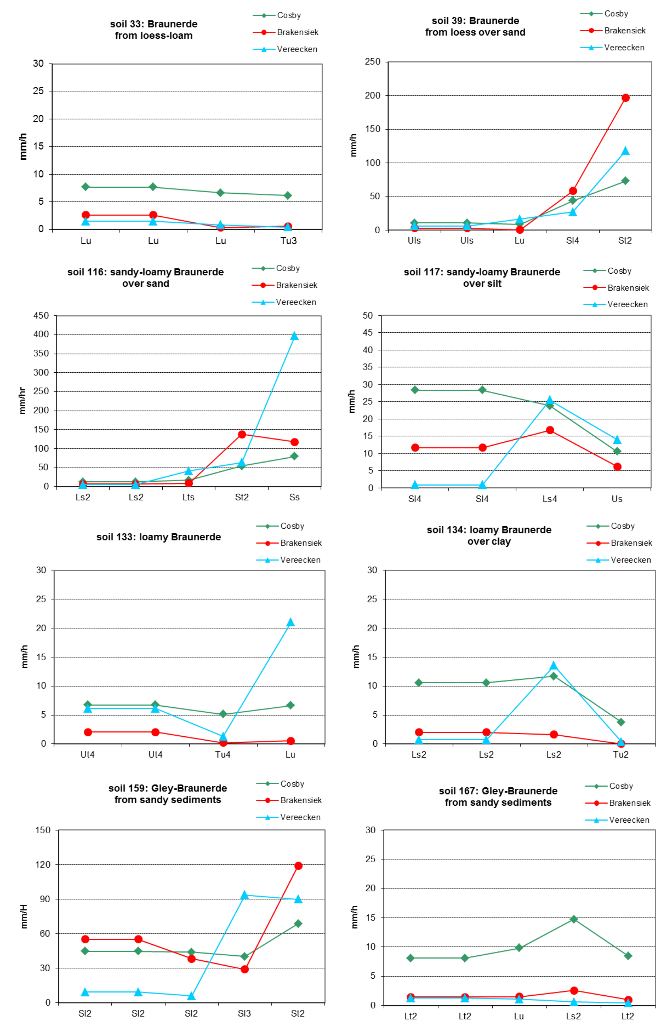
[fig:Estimation_saturated_conductivity]
| Bulk density Texture class | 1.3 | 1.4 | 1.5-1.6 | 1.7-1.75 | 1.8-1.9 | 2.0-2.1 | 2.3-2.4 |
|---|---|---|---|---|---|---|---|
| Table – Continued from previous page | |||||||
| Bulk density Texture class | 1.3 | 1.4 | 1.5-1.6 | 1.7-1.75 | 1.8-1.9 | 2.0-2.1 | 2.3-2.4 |
| mS | 200 | 125 | 125 | 83.4 | 83.4 | 42 | |
| fS | 83.4 | 42 | 29 | 16.7 | 10 | 4.2 | |
| Su,Slu | 29 | 16.7 | 10.4 | 4.2 | 2.3 | 0.4 | |
| Sl2 | 83.4 | 42 | 29.2 | 16.7 | 10.4 | 4.2 | |
| Sl3,Sl4,St2 | 83.4 | 42 | 29.2 | 16.7 | 10.4 | 2.3 | |
| St3 | 29.2 | 16.7 | 10.4 | 4.2 | 2.3 | 0.4 | |
| U,Us,Uls,Ul2, Ul3,Ut2,Ut3 | 29.2 | 16.7 | 10.4 | 4.2 | 2.3 | 0.2 | |
| Ul4,Ut4 | 42 | 16.7 | 10.4 | 4.2 | 2.3 | 0.2 | |
| Ls2,Ls3,Ls4 | 83.4 | 41.7 | 16.7 | 4.2 | 2.3 | 0.2 | |
| Lu | 29.2 | 16.7 | 10.4 | 4.2 | 2.3 | 0.2 | |
| Ltu | 83.4 | 42 | 16.7 | 4.2 | 2.3 | 0.2 | |
| Lts,Lt2,Lt3 | 42 | 16.7 | 10.4 | 4.2 | 2.3 | 0.2 | |
| Tu3,Tu4,Tl,Tu2,T | 42 | 16.7 | 10.4 | 4.2 | 2.3 | 0.2 | 0.1 |
| Hh | 83.4 | 16.7 | 10.4 | 4.2 | 2.3 | 0.2 | |
| Hn | 125 | 42 | 29.2 | 16.7 | 10.4 | 4.2 |
| [tab:Estimation_of_saturated_conductivity_KA4] | |||
|---|---|---|---|
| Soil texture class | Bulk density <1.6 SC [mm/h] | Bulk density = 1.6-1.8 SC [mm/h] | Bulk density >1.8 SC [mm/h] |
| Table – Continued from previous page | |||
| Soil texture class | Bulk density <1.6 SC [mm/h] | Bulk density = 1.6-1.8 SC [mm/h] | Bulk density >1.8 SC [mm/h] |
| Ss | 145.4 | 95.4 | 52.5 |
| Sl2 | 45.4 | 20.4 | 15 |
| Sl3 | 19.6 | 13.8 | 6.3 |
| Sl4 | 17.9 | 8.8 | 5 |
| Slu | 17.1 | 4.6 | 3.3 |
| St2 | 37.9 | 32.9 | 15.4 |
| St3 | 11.6 | 7.1 | 2.9 |
| Su2 | 65.4 | 36.7 | 15 |
| Su3 | 31.3 | 13.3 | 7.1 |
| Su4 | 17.1 | 10 | 8.3 |
| Ls2 | 17.1 | 8.3 | 5.4 |
| Ls3 | 5.4 | 2.9 | 2.5 |
| Ls4 | 8.3 | 5.8 | 2.5 |
| Lt2 | 5.4 | 3.8 | 1.7 |
| Lt3 | 4.2 | 4.2 | 2.9 |
| Lts | 5 | 2.5 | 1.3 |
| Lu | 10.8 | 7.5 | 2.5 |
| Uu | 6.7 | 2.9 | 1.2 |
| Uls | 14.6 | 5.8 | 2.1 |
| Us | 9.2 | 4.2 | 1.6 |
| Ut2 | 12.5 | 2.9 | 1.7 |
| Ut3 | 15.8 | 3.3 | 1.3 |
| Ut4 | 12.9 | 3.8 | 1.7 |
| Tt | 2.9 | 0.8 | 0.4 |
| Tl | 4.2 | 1.3 | 0.4 |
| Tu2 | 8.3 | 2.1 | 0.4 |
| Tu3 | 11.3 | 5.4 | 2.5 |
| Tu4 | 14.2 | 11.7 | 3.3 |
| gSfs | 153.8 | 54.2 | 20.8 |
| mS | 272.1 | 177.9 | 79.1 |
| mSgs | 242.1 | 117.1 | 29.1 |
| mSfs | 129.6 | 92.1 | 54.1 |
| fS | 71.7 | 44.2 | 16.6 |
| fSms | 101.7 | 70.4 | 25 |
| Hhz1 | 83.3 | 10.4 | 2.1 |
| Hhz2 | 83.3 | 10.4 | 2.1 |
| Hhz3 | 10.4 | 2.1 | 0.2 |
| Hhz4 | 2.1 | 0.2 | 0 |
| Hhz5 | 2.1 | 0.2 | 0 |
| nHv | 83.7 | 10.8 | 2.5 |
| nHm | 83.7 | 10.8 | 2.5 |
| nHa | 83.7 | 10.8 | 2.5 |
| nHt | 83.7 | 10.8 | 2.5 |
| nHr | 83.7 | 10.8 | 2.5 |
4.3.4 Crop Parameters and Crop Management Data
Crop parameters file crop.dat has to be included in the model input. It is a standard input file for SWIM. The full description of this data is given in Section 3.3.6.
Crop management data include description of agricultural activities:
day of operation,
operation code (planting, harvesting),
crop number (from the available crop data base, which also include some aggregated categories),
days of fertilisation,
amount of N and P in kg applied per hectare.
Cop management input in the model is not fully automatized at the moment. Therefore, the subroutine initcrop() has to be recompiled for new applications to take into account crop rotation and crop management. Three options are available for crop rotation now:
one crop in cropland,
10-11 years rotation scheme, including six crop types and set aside,
three different rotation schemes for three soil groups (poor, intermediate and high quality soils) with a stochastic crop distributor, so that crop rotation is the same within the soil group, but it is not synchronized for different ‘fields’ (starting year is choosen stochastically for the ‘fields’).
Later, this routine has to be rearranged to allow fully automatized climate data input.
4.3.5 Hydrological and water quality data
Additionally, river discharge and concentrations of nitrogen, phosphorus and suspended solids in the basin outlet are needed for model validation. River discharde has to be included in the model input (see format in ), while the measured water quality data can be compared with the model output outside the model.
| Table – Continued from previous page | |||
|---|---|---|---|
| YYYY | MON | DAY | Q,m3/s |
| 1981 | 1 | 1 | 3.10 |
| 1981 | 1 | 2 | 3.45 |
| 1981 | 1 | 3 | 7.92 |
| 1981 | 1 | 4 | 13.80 |
| 1981 | 1 | 5 | 6.81 |
| 1981 | 1 | 6 | 5.39 |
| 1981 | 1 | 7 | 4.86 |
| 1981 | 1 | 8 | 4.53 |
| 1981 | 1 | 9 | 4.13 |
| 1981 | 1 | 10 | 4.09 |
| 1981 | 1 | 11 | 3.97 |
| 1981 | 1 | 12 | 4.06 |
| .... | .. | .. | .... |
4.3.6 DEMO data set
DEMO data set is located in swim99/inpdata/clim – climate input data, swim99/inpdata/soil – soil input data, swim99/inpdata/crop – crop input data, swim99/inpdata/qwq – hydrological and water quality input data.
4.4 Model Run
4.4.1 Collect all input data
All input files necessary for the model application were listed in and described in . Their preparation is described in – . Here a summary is given on how to collect all prepared data before running SWIM.
The working directory (later called ‘main working directory’) is usually named by the basin name, It must have the following subdirectories: /Code – for the model code /Sub – for subbasin parameter files /Soil – for soil data files, /Struc – for subbasin structure files, /Res – for general model results, /Flo – for specific results on water and nutrient flows, /GIS – for specific results in GRASS GIS format, /Clim – for climate and hydrological data files.
After that all prepared files have to be copied in appropriate subdirectories as described below.
Step1. Files created by SWIM/GRASS interface The four files created by SWIM/GRASS interface in the user GRASS directory DATABASE/LOCATION/MAPSET/swim/projectname file.cio, str.cio, xxx.fig , xxx.str have to be copied to the main working directory.
The subbasin files created by SWIM/GRASS interface in the user GRASS directory DATABASE/LOCATION/MAPSET/swim/projectname xxxNN.sub – M files, where M is the number of subbasins, xxxNN.gw – M files, where M is the number of subbasins, xxxNN.rte – M files, where M is the number of subbasins have to be copied in the directory /Sub.
Step 2. Climate and hydrological data Climate and hydrological data have to be copied to the main working directory: either one file clim.dat, which includes all climate and hydrological data (see and ), or four files prec.dat, temp.dat, radi.dat, runoff.dat, which include separately precipitation, temperature, radiation, and runoff data, respectively. The directory /Clim may be used for original climate data sets and for climate data modification (e.g. to prepare two separate climate data sets for the calibaration and validation periods).
In the case of large number of subbasins and direct correspondence ‘1 subbasin – 1 precipitation station’, the file sub2prst.dat
may be prepared, which indicates the correspondence between subbasins and precipitation stations. If necessary, this file may contain weighting coefficients for precipitation stations. This file has to be placed in the main working directory.
Usually the climate read part is organised specifically for the basin under study by user (file cliread.f in the directory /Code), who can specify whether the datra are read from one file clim.dat, or from several files, and how the correspondence between subbasins and precipitation/climate stations is established.
Step. 3 Soil data The user has either use available soil database BÜK-1000 supplied with the model or to prepare all soil data in the same format as described in . Soil data soil04.dat, soil05.dat, etc Have to be copied in the directory /Soil. In addition, the file soil.cio, which includes a list of all soil data file names, has to be copied to the main working directory or prepared.
Step 4. Crop data The standard crop database contained in the file crop.dat, which is supplied with the model, has to be copied to the main working directory.
Step 5. Files .cod and .bsn An example program codes file xxx.cod, which includes program codes for printing, is supplied with the model. The user has to specify the desired period of simulation (parameters nbyr, iyr, idaf, idal), which has to be in correspondence with climate and hydrological data, and the number of subbasins (parameter lu). The print codes have to established by user, if the hydrotope printout, subbasin printout, process printout, or special printout are necessary. This file has to be placed in the main working directory.
An example basin parameters file xxx.bsn, which includes a set of basin parameters and a set of calibration parameters, is supplied with the model. The user has to introduce the correct basin area (parametr da), which can be taken from .bsn file produced by SWIM/GRASS interface. This file has to be placed in the main working directory.
Step 6. File wstor.dat An example file wstor.dat, which includes initial water storages for the reaches is supplied with the model. Here all initial storages may be put to 0, then initial period (1-2 weeks) of simulation has to be ignored. The other option is to take water storage at the end of the first year from the test model run. This file has to be placed in the main working directory.
Step 7. File wgen.dat An example file with monthly statistical climate data wgen.dat, is used to run weather generator. Besides this file is needed to establish rain intensity parameters (tp5, tp6, tp24), latitude (parameter ylt), and average monthly maximum and minimum temperature (vectors obmx, obmn). It is assumed that these parameters are basin-specific. The vectors obmx, obmn can be calculated using an additional program wgenpar from the available climate data, taking as long time series of climate for the basin as possible. Then the calculated average monthly maximum and minimum temperatures have to be substituted into the example wgen.dat file. The file wgen.dat has to be placed in the main working directory.
4.4.2 Modification of the code to adjust for specific input data
When all input data are ready, the user has to copy the source code files
| clicon.f | gwat.f | readcrp.f |
| cliread.f | hydrotop.f | readsol.f |
| common.f | init.f | readsub.f |
| compar.f | initcrop.f | readwet.f |
| crop.f | main.f | route.f |
| cropyld.f | ncycle.f | routfun.f |
| curn.f | open.f | solt.f |
| eros.f | pcycle.f | stat.f |
| evap.f | perc.f | subbasin.f |
| flohyd.f | readbas.f | veget.f |
| genres.f | readcod.f | vegfun.f |
and the Makefile from the supplied model package. Some files, which provide initialization of the model, may be corrected. The correction may be needed in
climate data read part (files open.f, and cliread.f),
crop initialization part (file initcrop.f),
soil parameter read part (file readsol.f),
global model parametre part (file modpar.f).
As soon as a certain flexibility is allowed regarding the climate data input, the corresponding changes may be necessary in files open.f, and cliread.f Different options are possible: from the simplest variant, when all climate and hydrological data are put in one file clim.dat, to another variant, when precipitation, tmeperature, radiation, and water discharge are put in four different files prec.dat, temp.dat, radi.dat, runoff.dat. Correspondingly, the assignment of precipitation stations to subbasins may be done differently. Examples are given in cliread.f.variants file located in /Codevar directory (supplied with the model).
Crop management is initialized in the file initcrop.f. Different options are possible in initialization of crop management:
single crop on the total cropland area,
different crop rotations and fertilization schemes,
crop generator.
The first two options may be used by including desired version of initcrop() subroutine. Examples are given in initrcrop.f.rotNferN and initcrop.f.single files located in /Codevar directory (supplied with the model). They can be used directly by opening the desired variant of initcrop() and closing the others. The user has to keep in mind that winter crops may start only from the second year of simulation (planting in autumn). That is why the single crop variants with winter crops include summer barley for the first year of simulation.
The third option (crop generator) is usually applied only for regional studies. It requires more changes in the code, and is supplied as a separate model version.
The user may either use the available soil database BÜK-1000, or another soil parameters. In principle, the format should be the same, then no changes are needed in the readsol.f file. In case if a new format is used, the corresponding changes have to be made in the file readsol.f Two examples: readsol.f.elbe and readsol.f.glonn are given in the /Codevar directory for the Elbe and Glonn basins, respectively.
Besides, the user may changes global model parameters, like maximum number of subbasins, mb, and maximum number of hydrotopes, meap, in the file compar.f This is necessary if the maximum number of subbasins/hydrotopes for the case study basin is larger than in the code, and it is also useful if the maximum number of subbasins/hydrotopes for the case study basin is significantly smaller than in the code (saves compilation time!).
4.4.3 Sensitivity of the simulated river discharge to model parameters
Sensitivity of the simulated river discharge to model parameters is one of the most important sensitivity studies with SWIM as an ecohydrological model. The results of sensitivity analysis are partly basin-specific, because they depend on the basin structure (land use, soil, tc.). The sensitivity study like one described in this chapter can be recommended for an unexperienced user in order to gain understanding of the model performance.
In this Section the results of sensitivity analysis made for the Stepenitz basin are presented. They are summarized in the following Table and Figures 4.7 – 4.25.
| Method to define saturated conductivity sc | Reference: sc calculated (Brackensiek method) | sc read from database |
|---|---|---|
| Model parameter used | isc = 1 | isc = 0 |
| Change in water balance | 6.0% | |
| Change in peaks | Peaks \(\uparrow\) \(\uparrow\) | |
| Change in level | Level \(\downarrow\) \(\downarrow\) |
| Correction of saturated conductivity sc, if sc is read (isc = 0) | Reference: | ||
|---|---|---|---|
| Model parameter used | sccor =1.2 | sccor = 1. | sccor = 0.8 |
| Change in water balance | -1.3% | 1.6% | |
| Change in peaks | Peaks \(\downarrow\) | Peaks \(\uparrow\) | |
| Change in level |
| Correction of saturated conductivity sc, if sc is calculated (isc = 1) | Reference: | ||
| Model parameter used | sccor =1.2 | sccor = 1. | sccor = 0.8 |
| Change in total water discharge | -1.0% | 1.2% | |
| Change in peaks | Peaks \(\downarrow\) | Peaks \(\uparrow\) | |
| Change in level | Level \(\uparrow\) | Level \(\downarrow\) |
| Soil depth | Reference: Soil depth is established according to maximum root depth | Soil depth is established according to maximum root depth + 50% |
|---|---|---|
| Change in total water discharge | -10.1% | |
| Change in peaks | Peaks \(\downarrow\) \(\downarrow\) | |
| Change in level | Level \(\downarrow\) \(\downarrow\) |
| Hydrological soil groups | Reference: soil groups A, B, C, D | A \(\rightarrow\) B, B \(\rightarrow\) C, C \(\rightarrow\) D, D = D | A \(\rightarrow\) C, B \(\rightarrow\) C, C \(\rightarrow\) D, D = D |
|---|---|---|---|
| Model parameter used | nsolgr = 1, 2, 3, 4 | nsolgr = 2, 3, 4, 4 | nsolgr = 3, 3, 4, 4 |
| Change in total water discharge | 0.30% | 0.90% | |
| Change in peaks | Peaks \(\uparrow\) | Peaks \(\uparrow\) \(\uparrow\) | |
| Change in level | Level \(\downarrow\) | Level \(\downarrow\) |
| Curve number method: differentiate on land use and soil or not | Reference: CN different, icn = 0 | icn = 1 | icn = 1 | icn = 1 | icn = 1 | icn = 1 | icn = 1 | icn = 1 |
|---|---|---|---|---|---|---|---|---|
| Model parameter used: cnum1, cnum3 | 30, 70 | 40, 80 | 50, 90 | 30, 80 | 40, 90 | 40, 70 | 50, 80 | |
| Change in total water discharge | -5.5% | -5.5% | -5.0% | -5.5% | -5.1% | -5.5% | -5.5% | |
| Change in peaks | Peaks \(\downarrow\) no small peak s | Peaks \(\downarrow\) no small peaks | Peaks \(\uparrow\) no small peaks | Peaks \(\downarrow\) no small peaks | Peaks \(\uparrow\) no small peaks | Peaks \(\downarrow\) no small peaks | Peaks \(\downarrow\) no small peaks | |
| Change in level | no | no | no | no | no | no | no |
| Baseflow factor for return flow travel time | Reference | |||||
|---|---|---|---|---|---|---|
| Model parameter used: bff | bff = 1. | bff = 1.5 | bff = 2. | bff = 3. | bff = 0.5 | bff = 0.2 |
| Change in total water discharge | 1% | 1.6% | 2.3% | -1. 5 % | -3.4% | |
| Change in peaks | Peaks \(\uparrow\) | Peaks \(\downarrow\) | ||||
| Change in level | Level \(\downarrow\) | Level \(\uparrow\) |
| Alpha factor for groundwater | Reference | ||||
|---|---|---|---|---|---|
| Model parameter used: abf0 | abf0 = 0.048 | abf0 = 0.1 | abf0 = 0.3 | abf0 = 0.024 | abf0 = 0.012 |
| Change in total water discharge | 1% | 1.7% | -1.4% | -3.5% | |
| Change in peaks | Peaks \(\uparrow\) in winter-spring | Peaks \(\downarrow\) in winter-spring | |||
| Change in level | Level \(\uparrow\) in winter-spring | Level \(\downarrow\) in winter-spring |
| Initial groundwater contribution to flow | Reference | ||
|---|---|---|---|
| Model parameter used: gwq0 | gwq0 = 0.5 | gwq0 = 0.2 | gwq0 = 1. |
| Change in total water discharge | -5.1% | 8.4% | |
| Change in peaks & level | Initial peaks and level \(\downarrow\) | Initial peaks and level \(\uparrow\) |
| Initial soil water storage | Reference | ||
|---|---|---|---|
| Model parameter used: stinco | stinco = 0.7 | stinco = 0.4 | stinco = 1.0 |
| Change in total water discharge | -3.4% | 3.1% | |
| Change in peaks & level | Initial peaks and level \(\downarrow\) | Initial peaks and level \(\uparrow\) |
| Routing coefficients | |||||||
|---|---|---|---|---|---|---|---|
| Model parameter used: roc2, roc4 | 3, 3 | 6, 6 | 12, 12 | 24, 24 | 48, 48 | 6, 48 | 96, 96 |
| Change in total water discharge | 0% | -0.2% | -0.6% | -1.2% | -1% | -2.2% | |
| Change in peaks | Peaks \(\downarrow\), dynamics - smoother | Peaks \(\downarrow\), dynamics - smoother | Peaks \(\downarrow\), dynamics - smoother | Peaks \(\downarrow\), dynamics - smoother | Peaks \(\downarrow\), dynamics - smoother | Peaks \(\downarrow\), dynamics - smoother |
| Crop type (in the case if only one crop type on cropland) | Reference: winter rye | winter wheat | winter barley | summer barley | maize | potatoes |
|---|---|---|---|---|---|---|
| Model parameter used: ncrp | ncrp =iwr | ncrp =iww | ncrp =iwb | ncrp =isba | ncrp =imai | ncrp =ipo |
| Change in total water discharge | -3.0% | -2.2% | 0.4% | -0.9% | 1.2% | |
| Change in peaks | some peaks - different | some peaks - different | some peaks - different | some peaks - different | some peaks - different |
4.4.4 Overview of SWIM applications
Model validation SWIM was tested and validated sequentially for hydrological processes, for nitrogen dynamics, crop growth and erosion. First validation for hydrological processes performed for several mesoscale river basins is described in . Preliminary validation of the model for nitrogen dynamics and crop growth is described in . First test for erosion processes was performed for the Mulde basin (area 6171 km2), and it is described in . More detailed validation of the model for hydrological processes and nitrogen dynamics in the lowland and mountainous sub-regions of the Elbe was done for the Stepenitz and the Zschopau basins . These two papers include also the analysis of factors affecting nitrogen export from diffuse agricultural sources of pollution. More elaborate validation of the erosion processes in SWIM was done for the Glonn basin in Bavaria (392 km2, ), where more detailed data than for the Mulde basin were available. Results of the model validation are quite satisfactory. Further development is foreseen for some processes, like nutrient retention in river basins. Besides the validation studies, the model was applied for the land use change and climate change impact studies, which are described below.
Land use change impact study was performed for the state of Brandenburg, Germany. Besides general vulnerability against water stress due to natural conditions, water resources in Brandenburg are strongly affected by brown coal mining, which took place in the south-east of the federal state in the last decades. Now the mining activities are significantly shortened. This results in decreasing river discharge, in particular in the Spree river, and may lead to general shortages in water availability. Land use change is one possible option to counteract this development.
As regards land use change trends, a tendency towards deintensification in the use of agricultural land is observed in Brandenburg during the last decade. The increase in a temporary set-aside within crop rotations was the main measure used to decrease the intensification level on arable land. Another effective way to deintensify crop production and, at the same time, to protect environmentally sensitive areas, is to create buffer zones along river courses (river corridors) by converting the arable land there into grassland or forest (permanent “set-aside”). Besides, the latter is an efficient way to reduce nitrate pollution and sediment load in rivers and to improve water quality.
Therefore, the primary objective of our study was to analyse the effects of these two alternatives of deintensification in the use of arable land on water resources in Brandenburg. Three types of land use change scenarios were developed and applied: - modification of the basic rotation scheme by increasing the portion of temporary “set-aside”; - introducing river corridors (150 and 500m width) in the original land use map and converting cropland within them into meadows (permanent “set-aside”); - combinations of temporary and permanent set-aside schemes described above.
Two opposite tendencies were established in our simulation study. The temporary “set-aside” within a crop rotation scheme would result in decreasing evapotranspiration and increasing runoff and groundwater recharge in the region, whereas the permanent set-aside within river corridors would reduce runoff and increase evapotranspiration.
Therefore, land use changes in terms of deintensification may compensate for the expected decrease of discharge in the river Spree over the coming period, only if these changes assume increases in the portion of temporary set-aside areas, and do not include conversion of arable land into meadows (or forests). Runoff increases might be even greater with a decreasing production intensity on the remaining area for arable crops, due to reduction in regional transpiration as consequence of the lowered leaf area index. The land use change impact study is described in , and .
Climate change impact The analysis of climate change impacts on hydrology and crop yield was performed also for the state of Brandenburg, applying two transient 1.5 K scenarios of climate change. In advance, hydrological validation was performed in three representative mesoscale river basins in the area, and the crop module was validated regionally for Brandenburg, using crop yield data for districts. The CO2 fertilization effect was studied in two options, considering: a) adjustment of the potential growth rate per unit of intercepted PAR by a temperature dependent correction factor alpha based on experimental data for C3 and C4 crops; b) assuming a CO2 influence on transpiration at the regional scale as the beta factor, which is coupled to the factor alpha.
Two transient 1.5 K scenarios of climate change for Brandenburg were developed in PIK: wet scenario W15 and dry scenario D15. Three periods were compared: 1981 - 1992 (control period A), 2022 - 2030 (period B), and 2042 - 2050 (period C). The atmospheric CO2 concentration for the reference period and two scenario periods were set to 346, 406 and 436 ppm, respectively. According to the scenario W15, precipitation is expected to increase in Brandenburg: +5.2% and +11.7% on average in periods B and C, respectively. According to the scenario D15, precipitation is expected to decrease slightly in the period B (-1.7%) and quite significantly in the period C (-11.3%).
Evapotranspiration is expected to increase quite significantly under changing climate for the scenario W15, and moderately for the scenario D15. Groundwater recharge is practically the same as that in the control period for scenario W15. On the opposite, the decrease of groundwater recharge is notable for scenario D15, down to -31.5% in the period C. According to scenario W15, runoff is increasing (up to +17.2% in the period C). However it decreases significantly in the period C for scenario D15 (-22.6%).
The crop yield was only slightly altered under the "climate change only" variant of the W15 scenario for barley and maize, and it was reduced for wheat. The D15 scenario lead to the reduced crop yield for all the crops.
The impact of higher atmospheric CO2 (alpha factor) compensated fully or partly for climate-related crop yield losses, and resulted in an increased yield both for barley and maize in scenario W15 compared to the reference scenario. The negative changes were still preserved in scenario D15 for wheat and maize.
The assumption that in addition stomatal control of transpiration is taking place at the regional scale (beta factor coupled to alpha factor) lead to further increase in crop yield, which was larger for maize than for barley and wheat. A full description of the climate change impact study with scenario W15 is given in .
Conclusions One of the major challenges for BAHC (Biospheric Aspects of Hydrological Cycle) research in the frame of the International Geosphere and Biosphere Program (IGBP) is the adequate description and modelling of the complex interactions between climate, hydrological and ecological processes at different scales. SWIM has been developed as a tool to serve this purpose at the mesoscale and regional scale.
Model applications in a number of river basins in the range of about 100 to 24000 km2 drainage area have shown that the model is capable to describe realistically the basic ecohydrological processes under different environmental conditions, including a) the spatial and temporal variability of main water balance components (evapotranspiration, groundwater recharge, runoff generation), b) the cycling of nutrients in soil and their transport with water considering the dynamics of the controlling climate and hydrological conditions, c) vegetation/crop growth and related phenomena, d) the dynamical features of soil erosion and sediment transport, and e) the effect of changes in climate and land use on all these interrelated processes and characteristics.
4.5 Output variables
| name | description | unit |
|---|---|---|
| baseflow | mm | |
| biomass_total | ||
| crop_yield | ||
| discharge | \(m^3s^{-1}\) | |
| eta | mm | |
| etp | mm | |
| glacier_weq | m | |
| groundwater_recharge | mm | |
| heat_unit_fraction | ||
| leaf_area_index | ||
| percolation | mm | |
| precipitation | mm | |
| river_runoff | mm | |
| root_depth | ||
| snow_depth_weq | ||
| snowfall_weq | mm | |
| soil_evaporation | mm | |
| soil_water_content | mm | |
| soil_water_index | ||
| subsurface_runoff | mm | |
| surface_runoff | mm | |
| tmax | ||
| tmean | ||
| tmin | ||
| transpiration | mm | |
| vegetation_temperature_stress | ||
| vegetation_water_stress | ||
| water_yield |
5 APPENDIX I GRASS commands useful for the spatial data preparation for SWIM
| Command format | Flags and Parameters | Command description |
|---|---|---|
| Table – Continued from previous page | ||
| Command format | Flags and Parameters | Command description |
| d.colors | Parameters: map raster map name | To interactively change the color table of a raster map layer |
| d.display | A menu-driven display program for viewing maps | |
| d.erase | Parameters: color color to erase with | Erases the contents of the active display frame on the user’s monitor |
| d.frame [-cepsD] | Flags: -c Create a new frame -e Remove all frames and erase the screen -p Print name of current frame -s Select a frame -D Debugging output Parameters: frame frame to be created/selected at where to place the frame | Manages display frames on the user’s monitor |
| d.histogram [-zq] map=name | Flags: -z Display zero-data information -q Gather the histogram quietl Parameters: map raster map for which histogram will be displayed color color for legend and title options: red, orange, yellow, green, blue, indigo, white, black, brown, magenta, aqua, gray, grey style indicate if a pie or bar chart is desired | Displays a histogram in the form of a pie or bar chart for a user-specified raster file |
| d.legend map=name | Parameters: map name of raster map color sets the legend’s text color llines number of text lines (useful for truncating long legends | Displays a legend for a raster map layer in the active frame on the graphics monitor |
| d.mon [-lLprs] | Flags: -l List all monitors -L List all monitors (with current status -p Print name of currently selected monitor -r Release currently selected monitor -s Do not automatically select when starting start name of graphic monitor to start Parameters: stop name of graphic monitor to stop select name of graphic monitor to select unlock name of graphic monitor to unlock | To establish and control the use of a graphics display monitor |
| d.rast [-o] map=name | Flags: -o Overlay (non-zero values only) Parameters: map name of raster map to be displayed | Displays and overlays raster map layers in the active display frame on the graphics monitor |
| d.vect [-m] map=name | Flags: -m Use less memory Parameters: map name of vector map to be displayed color color desired for drawing map | Displays vector data in the active frame on the graphics monitor |
| d.what.rast [-1t] ] | Flags: -1 Identify just one location -t Terse output. For parsing by programs. Parameters: map name of raster map(s) fs field separator (terse mode only), default: : | Allows the user to interactively query the category contents of multiple raster map layers at user-specified locations within the current geographic region |
| d.what.vect [-1] map=name | Flags: -1 Identify just one location Parameters: map name of existing vector map | Allows the user to interactively query the category contents of a (binary) vector map layer at user-specified locations within the current geographic region |
| d.where [-1] | Flags: -1 one mouse click only Parameters: sspheroid name of a spheroid for lat/lon coordinate conversion, options: australian, bessel, clark66, everest, international, wgs72, wgs84 | Identifies the geographic coordinates associated with point locations in the active frame on the graphics monitor |
| d.zoom [-q] | Flags: -q Quiet Parameters: action type of zoom (for latitude/longitude databases only) options: zoom, rotate | Allows the user to change the current geographic region settings interactively, with a mouse |
| r.average [-c] base=name cover=name output=name | Flags: -c cover values extracted from the category labels of the cover map Parameters: base base raster map cover cover raster map output resultant raster map | Finds the average of values in a cover map within areas assigned the same category values in a user-specified base map |
| r.buffer [-q] input=name output=name distances=value[,value,...] | Flags: -q Quiet Parameters: input name of input map output name of output map distances distance zone(s) units units of distance, options: meters, kilometers, feet, miles, default: meters | Creates a raster map layer showing buffer zones surrounding cells that contain non-zero category values |
| r.cats map=name ] | Parameters: map name of a raster map cats category list: e.g. 1,3-8,14 fs output separator character, default: tab | Prints category values and labels associated with user-specified raster map layer |
| r.coin [-qw] map1=name map2=name units=name | Flags: -q Quiet -w Wide report, 132 columns (default: 80) Parameters: map1 name of first raster map map2 name of second raster map units unit of measure, options: c,p,x,y,a,h,k,m | Tabulates the mutual occurrence (coincidence) of categories for two raster map layers |
| r.colors [-wq] map=name color=type | Flags: -w Don’t overwrite existing color table -q Quietly Parameters: map raster map name color type of color table options: aspect, grey, grey.eq, gyr, rainbow, ramp, random, ryg, wave, rules Where color type is one of: aspect (aspect oriented grey colors) grey (linear grey scale) grey.eq (histogram equalized grey scale) gyr (green through yellow to red) rainbow (rainbow color table) ramp (color ramp) ryg (red through yellow to green) random (random color table) wave (color wave) rules (create color table by rules) Valid colors are: white black red green blue yellow magenta cyan aqua grey gray orange brown purple violet indigo | Creates/modifies the color table associated with a raster map layer |
| r.combine [-s] | Flags: -s Use symbols (instead of graphics | Allows category values from several raster map layers to be combined |
| r.cross [-qz] input=name[,name,...] output=name | Flags: -q Quiet -z Non-zero data only Parameters: input names of 2-10 input raster maps output name of the resulting map | Creates a cross product of the category values from multiple raster map layers |
| r.describe [-1rqd] map=name | Flags: -1 Print the output one value per line -r Only print the range of the data -q Quiet -d Use the current region Parameters: map name of raster map | Prints terse list of category values found in a raster map layer |
| r.in.ascii input=name output=name | Parameters: input ascii raster file to be imported output name of resultant raster map title title for resultant raster map mult multiplier for ascii data, default: 1. | Convert an ASCII raster text file (e.g., from ARC/INFO) into a binary raster map layer |
| r.info map=name | Parameters: map name of raster map | Outputs basic information about a user-specified raster map layer |
| r.mapcalc | Raster map layer data calculator, performs arithmetic operations on several raster map layers | |
| r.neighbors [-aq] input=name output=name method=name size=value | Flags: -q Run quietly -a Do not align output with the input Parameters: input name of existing raster file output name of the new raster file method neigborhood operation, options: average, median, mode, minimum, maximum, astdev., variance, diversity, interspersion size neigborhood size, options: 1,3,5,7,9,11,13,15,17,19,21,23,25 title title of the output raster file | Makes each cell category value a function of the category values assigned to the cells around it, and stores new cell values in an output raster map layer |
| r.out.ascii [-h] map=name | Flags: -l Smooth Corners | Converts a raster map layer into an ASCII text suitable for other computer systems (e.g., for ARC/INFO) |
| r.poly [-l] input=name output=name | Flags: -h Suppress printing of header information Parameters: map name of existing raster map digits the minimum number of digits per cell to be printed | Extracts area edges from a raster map layer and converts data to GRASS vector format |
| r.reclass input=name output=name | Parameters: input raster map to be reclassified output name for the resulting raster map title title for the resulting raster map | Creates a new map layer whose category values are based upon the user’s reclassification of cate-gories in an existing map |
| r.report map=name[,name,...] ] | Flags: -h suppress page headers -m report zero values due to mask -f use form feeds between pages -q quiet -e scientific format -z filter out zero category data Parameters: map raster map(s) to report on units mi(les), me(tres), k(ilometers), a(cres), h(ectares), c(cells), p(ercent) pl,pw page length, page width output name of an output file | Reports statistics for raster map layers |
| r.stats [-1aclmqzgx] input=name[,name,...] | Flags: -1 One cell per line -a Print area totals -c Print cell counts -l Print category labels -m Report zero values due to mask -q Quiet -z Non-zero data only will be output -g Print grid coordinates (east and north) (requires -1 flag) -x Print x and y (column and row) (requires -1 flag) Parameters: input raster maps(s) fs output field separator, default: space output output file name | Generates area statistics for raster map layers |
| r.watershed [-m4] elevation=name | Flags: -m Enable extend memory option: Operation is slow -4 Allow only horizontal and vertical flow of water Parameters: Input maps: elevation Input map: elevation on which entire analysis is based depression Input map: locations of real depressions flow Input map: amount of overland flow per cell disturbed.land Input map or value: percent of disturbed land, for RUSLE blocking Input map: terrain blocking overland surface flow, for RUSLE threshold Input value: minimum size of exterior watershed basin max.slope.length Input value: maximum length of surface flow, for RUSLE Output maps: accumulation Output map: number of cells that drain through each cell drainage Output map: drainage direction basin Output map: unique label for each watershed basin stream Output map: stream segments half.basin Output map: each half-basin is given a unique value visual Output map: useful for visual display of results length.slope Output map: slope length and steepness (LS) factor for RUSLE slope.steepness Output map: slope steepness (S) factor for RUSLE | Watershed basin analysis program. It generates a set of maps indicating the location of sub-basins and streams, and the LS and S factors of the Revised Universal Soil Loss Equation (RUSLE) |
| g.remove [rast=name[,name,...]] [vect=name[,name,...]] [icon=name[,name,...]] [labels=name[,name,...]] [sites=name[,name,...]] [region=name[,name,...]] [group=name[,name,...]] [3dview=name[,name,...]] | Parameters: rast rast file(s) to be removed vect vect file(s) to be removed icon icon file(s) to be removed labels labels file(s) to be removed sites sites file(s) to be removed region region file(s) to be removed group group file(s) to be removed 3dview 3dview file(s) to be removed | Removes data base element files from the user’s current mapset |
| g.rename | Parameters: rast rast file(s) to be renamed vect vect file(s) to be renamed icon icon file(s) to be renamed labels labels file(s) to be renamed sites sites file(s) to be renamed region region file(s) to be renamed group group file(s) to be renamed 3dview 3dview file(s) to be renamed | To rename data base element files in the user’s current mapset |
| p.map | Parameters: input file containing mapping instructions (or use input=- to enter from keyboard scale scale of the output map, e.g. 1:25000 (default: 1panel) | Hardcopy color map output utility |
6 New developments until 2015
Stefan Liersch
6.1 Introduction
In the last couple of years the eco-hydrological model SWIM (Soil and Water Integrated Model) was applied to many different river basins worldwide in order to study the impacts of changes in climate, land use, and water management. Challenged by new and sometimes rather specific requirements, the SWIM community developed approaches to answer these research questions. For example, to tackle land and water management issues, the reservoir, water allocation and irrigation, and crop rotation modules were developed. Moreover, climatic conditions in regions differing from Central Europe or the application to large river basins (up to 2.2 million km2) required adaptation of existing or the development of new functionalities, such as the snow and glacier module or the possibility to calibrate SWIM at the subcatchment scale.
These modules were implemented in different versions or branches of the SWIM model by different persons. Now, it was time to implement all those developments in the SWIM trunk or master version, giving the user the opportunity to use or not to use these new functionalities by switching modules on or off.
The purpose of this manual is to introduce the user briefly to the functionality of the different modules and to describe the required input files in detail.
Some output files have changed in their formatting and number of columns.
The asterisk (*) is a placeholder for the project name.
6.2 git SWIM repository
The SWIM code, documentation, and the control files are centrally stored in the swim.git repository on the PIK GitLab:
https://gitlab.pik-potsdam.de/swim/swim6.2.1 Clone repository from cluster to your local machine
In order to create a copy (clone) of the repository on your local machine, navigate to a directory (on the local machine) where you want the repository to be located. Execute:
git clone username@cluster.pik-potsdam.de:/data/swim/swim.gitreplace username by your PIK account name. This will create the entire repository (including the SWIM code, the documentation, and the example control files) in the given directory.
6.2.2 Create a new branch or use the master (trunk version)?
If you intend to develop new and specific functionalities in SWIM that are not supposed to be implemented in the master branch (trunk version), you should definately create a new branch. This might be the case, if you have to adapt the SWIM model to very specific requirements of your catchment. If you are going to work on the master branch (trunk version), e.g. to implement a new module into the SWIM trunk version or to fix a bug, you need to switch to the master branch (see Section ).
6.2.2.1 Creating a new branch
git checkout -b branchnameThis will create a new branch branchname of the SWIM repository on your local machine. The original files are base on the master branch.
6.2.2.2 Delete a branch
git branch -d branchnameThis will delete the branch branchname on your local machine.
6.2.2.3 Commit all your changes locally
To commit your changes on your local machine (without pushing them to the branch on the cluster), type the following:
git commit -a -m"your comment briefly describing the changes you made"This works similarly for commiting changes to your branch or the master (trunk version), depending on the branch you are currently logged in.
6.2.2.4 Switch between branches
You can switch between the master branch and any other branch with the checkout command. If you made changes in the current branch without committing them, you cannot switch branches. So, commit your changes first, otherwise they may get lost!
git checkout master
git checkout branchname
The first line would switch to the master branch (trunk version) and the second to the branch branchname.
6.2.2.5 Commit your local changes to your branch or the master branch on the cluster
git push -u origin branchnameIn case you are committing your changes to the master branch (trunk version), the branchname is master.
6.2.3 Some other useful git commands
To show in which branch you are currently in and the files that have been changed but not yet committed:
git status To open the graphical git repository browser:
gitk (only current branch)
gitk --all (shows all branches)
You may have to install gitk first. On Ubuntu Linux it is as simple as:
sudo apt-get install gitk6.2.4 Working on the SWIM documentation
If you are modifying the SWIM documentation (Latex file), you must always work in the master branch before you commit and/or push your changes! See Section how to switch to the master branch.
6.3 Input Files
6.3.1 swim.conf
6.3.2 Basin input file (*.bsn)
The *.bsn file (the asterisk stands for the project name) consists of basically two sections. The first section (lines 2-12) contains switch parameters used to switch specific modules or functions ON or OFF. The second section (lines 14-48) comprises global parameter settings, such as correction factors for calibration parameters. Note that not all of these values are always used by the model because some of them may be overwritten if the subcatch switch (subcatchment calibration) is used.
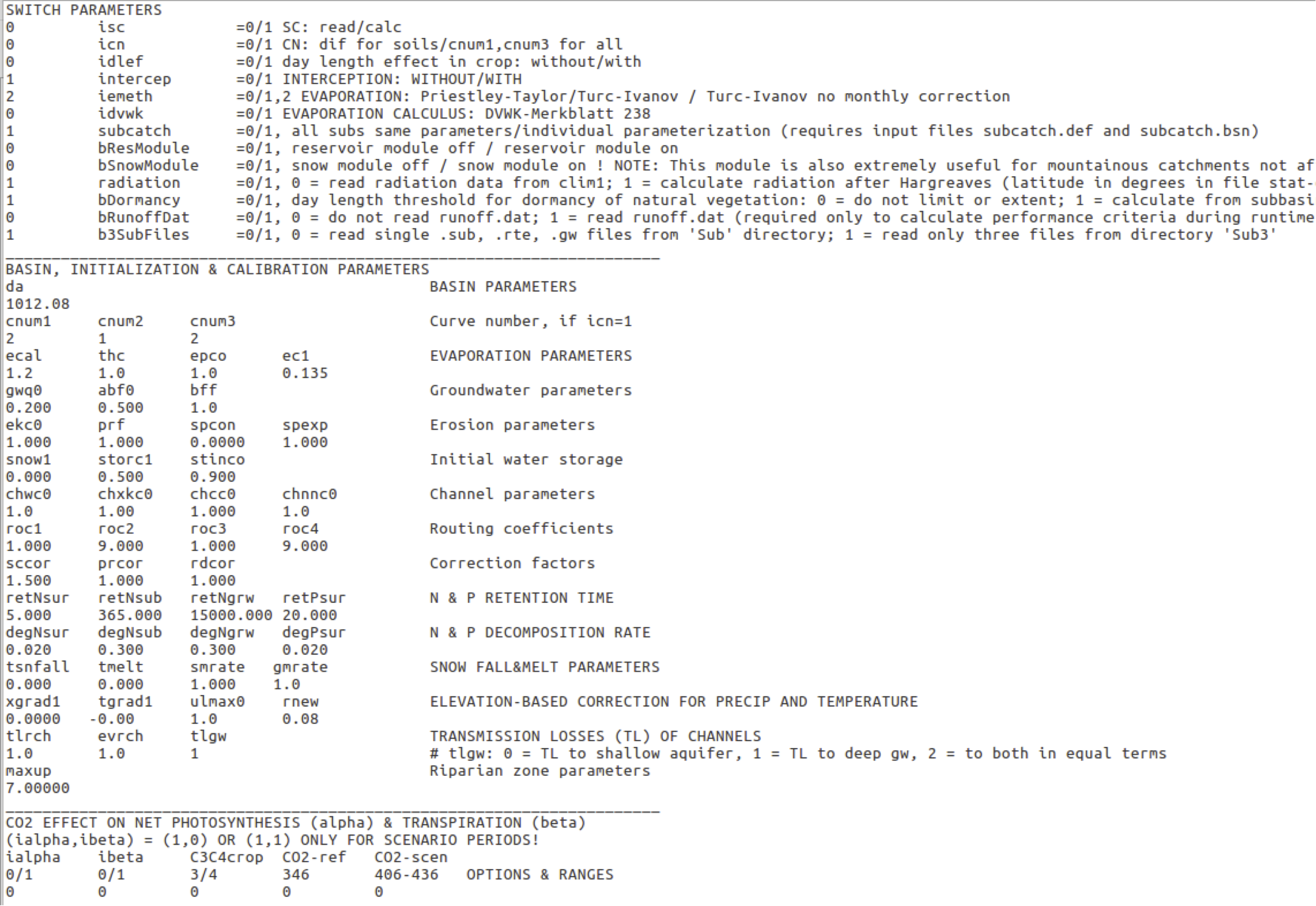
6.3.2.1 SWITCH parameters (*.bsn)
| Parameter | Description |
|---|---|
| Parameter | Description |
| isc | Soil saturated conductivity (read or calculate) |
| 0 = read saturated conductivity values from soil parameter files (recommended) | |
| 1 = calculate from clay content, sand content and porosity using the method of Brakensiek | |
| icn | Curve number values |
| 0 = read curve number values from *.lut (recommended) | |
| 1 = use curve number values cnum1, cnum2, cnum3 provided in the parameter section of the *.bsn file for all soils and land use categories | |
| idlef | Day length effect in crops. |
| 0 = with day length effect | |
| 1 = without day length effect | |
| intercep | Interception of vegetation canopy |
| 0 = no interception storage | |
| 1 = use interception storage (recommended) | |
| iemeth | Method to calculate potential evapotranspiration |
| 0 = Priestley-Taylor | |
| 1 = Turc-Ivanov (in this case, you may specify monthly correction factors for your catchment. The hardcoded values in evap.f are adapted to the Elbe catchment in Germany) | |
| 2 = Turc-Ivanov, but monthly correction deactivated! Monthly correction factor = 1.0 | |
| idvwk | Potential evaporation calculation according to DVWK-Merkblatt 238 |
| 0 = standard | |
| 1 = use DVWK method | |
| subcatch | Calibration of some global basin and ground water parameters at the entire basin scale (parameters valid for all subbasins) or at the subcatchment scale (individual settings for grouped subbasins), see Section for more detailed description and requirements. |
| 0 = using the same setting for all subbasins | |
| 1 = using different settings for grouped subbasins (subcatchments) | |
| landmgt | Crop management and rotations (initcrp.f) |
| 0 = using hardcoded crop rotations for all crop lands (land use ID = 5) | |
| 1 = using crop rotation scenarios defined in the external file landmgt.csv, see Section for a more detailed description and requirements. | |
| bResModule | Reservoir module, see Section for a more detailed description and its requirements. |
| 0 = not used | |
| 1 = used | |
| bSnowModule | Snow module, see Section for a more detailed description and its requirements. |
| 0 = not used | |
| 1 = used | |
| radiation | Read or calculate radiation data at subbasin scale, see Section for a more detailed description and its requirements. |
| 0 = reading radiation data from clim1.dat | |
| 1 = calculate radiation data after Hargreaves (1985), subroutine hargreaves_rad in readcli.f | |
| bDormancy | Determine dormancy period of natural vegetation |
| 0 = standard method for day length threshold | |
| 1 = modifying day length threshold based on subbasins’ latitude | |
| bRunoffDat | Input file runoff.dat is “only” used to calculate performance criteria during runtime and is most of the time not required. |
| 0 = do not read runoff.dat (file not required) | |
| 1 = read runoff.dat | |
| [tab:SWITCH_parameters] |
6.3.2.2 Global parameters (*.bsn)
| Parameter | Description |
| Parameter | Description |
| da | Basin area, \(km^2\). This is of course not a calibration parameter and should be calculated in GIS or from the *.str file as the sum of HRU areas. |
| cnum1, cnum2, cnum3 | Curve number values (only considered if icn = 1). It is recommended to use the land use-specific curve number values provided in *.lut file (see Section ) by setting icn = 0. |
| ecal 2) | Correction factor for potential evapotranspiration. Recommended range (0.7 - 1.3). |
| thc 2) | Correction factor for potential evapotranspiration on sky emissivity, range (0-1). 0 = without sky emissivity factor. |
| epco | Factor to limit plant water demand compensation from lower layers. If epco = 1.0, the compensation is not limited. |
| ec1 | Empirical constant in the Hargreaves & Samani (1985) equation used to calculate radiation. The parameter has only an effect, if radiation is calculated based on \(T_{min}\) and \(T_{max}\) (radiation switch = 1). NOTE: This parameter is very sensitive! And should probably be in the range of 0.1 and 0.2 |
| gwq0 1) | Initial ground water flow contribution to streamflow, mm/day. |
| abf0 1) | Alpha factor for grounwater. This parameter characterizes the ground water recession (the rate at which ground water flow is returned to the stream). |
| bff 1) | Base flow factor, used to calculate return flow travel time. |
| ekc0 | Soil erodibility correction factor. This parameter is used to correct all values ek() of soil erodibility obtained from soil database. |
| prf | Coefficient to estimate peak runoff in stream, used in calculation of sediment routing. |
| spcon | Rate parameter for estimating sediment transport (between 0.0001 and 0.01). |
| spexp | exponent for estimation of sediment transport (between 1. and 1.5). |
| snow1 | Initial snow content in the basin (mm). |
| storc1 | Initial water storage in streams correction coefficient. |
| stinco1 | Initial water content in the basin as a fraction of field capacity. |
| chwc0 | Coefficient to correct the channel width for all reaches. The channel width is estimated by GRASS interface. |
| chxkc0 | Correction coefficient for channel USLE K factor |
| chcc0 | Correction coefficient for channel USLE C factor |
| chnnc0 | Correction coefficient for channel Manning’s N factor |
| [tab:GLOBAL_BSN_parameters] |
6.3.3 *.cod
6.3.4 file.cio
6.3.5 Structure file (*.str)
HRU definition.
Created by GIS during the pre-processing.
Some specific modules require a column in the structure file (*.str), regardless whether they are used in the simulation or not. The structure of the *.str file is always the same.
Column 1 is the subbasin number, column 2 the land use ID, column 3 the soil ID, column 4 the land management ID, column 5 the wetland ID, the HRU elevation, column 6 the initial glacier depth, column 7 the HRU area, column 8 the number of cells and column 9 the irrigation ID.
6.3.6 *.lut (formerly cntab.dat)
The input file *.lut contains land use type-specific parameters. Four curve number values for the four soil hydrological groups, the maximum canopy storage for interception (mm) and the vegetation type (icnum) in the crop.dat (see Figure ).
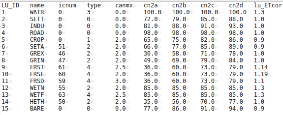
6.3.7 stat-outdat.csv
This new input file provides the latitude and and elevation for each subbasin. The latitude is required to calculate the day length for each subbasin individually instead of using the catchments’ average latitude from wgen.dat. This is particularly important for large river basin stretching from South to North, like the Nile basin, for instance.
The file consists of four columns (Subbasin ID, Longitude, Latitude, Elevation). This file is usually generated for interpolating the climate data to the subbasin centroids. But note that the coordinates used for interpolation are always in a metric geographic coordinate system like UTM or LAEA. The unit for longitude and latitude in this file have to be in decimal degree and the elevation in m.a.s.l.
6.3.8 runoff.dat
The runoff.dat can either be used to evaluate discharge simulations during runtime and/or to substitute simulated discharges in headwater subbasins with discharge observations. This is actually extremely useful for calibration. The runoff.dat has a header column (YEAR MONTH DAY \(obs_1...obs_n\)). The first column in the second row indicates the number of observation columns provided in this file. The values in the second and third column are only dummies (placeholder for columns MONTH and DAY) and can contain any integer number. The following columns indicate the subbasin numbers corresponding to the discharge gauges. Time series data of daily observed discharges start in the third row (see Table ).
| YEAR | MONTH | DAY | obs1 | obs2 |
| 2 | 0 | 0 | 110 | 120 |
| 1979 | 1 | 1 | 230.4 | 523.5 |
| 1979 | 1 | 2 | 233.5 | 526.3 |
| ... |
[tab:runoff.dat]
6.4 Modules
6.4.1 Subcatchment calibration
6.4.2 Crop management and rotations
6.4.3 Reservoir Module
6.4.4 Snow Module
6.4.5 Calculation of radiation data
New parameter ec1 in *.bsn file. ec1 represents an empirical constant in the Hargreaves (1985) equation. Appropriate values are probably between 0.1 and 0.2. But this needs to be varified from the publication.
6.4.6 Transmission losses
The calibration parameters tlrch and evrch in the *.bsn file can be used to account for transmission losses in the river bed (channel losses) and from the river surface area (evaporative losses), respectively. A value of 0.0 means no losses.
The parameter tlgw is used to determine to which ground water component the channel losses are attributed to. They can either be added fully to the shallow ground water storage (tlgw = 0, in this case the increasing shallow ground water storage can lead to increasing ground water contribution), fully to the deep ground water storage (tlgw = 1, in this case the water is lost from the system but appears in the water balance), or to both components in equal terms (tlgw = 2).
Due to the fact that the transmission losses are computed in the routing process (after the subbasin cycle), the losses are abstracted from the routed discharge. Hence, the possibly increasing actual evapotranspiration from the river water surface in the respective subbasin cannot be attributed to the subbasins’ actual evapotranspiration but it is accounted for in the water balance output files (bad.prn, bam.prn, bay.prn, and bay_sc.csv).
6.5 The SWIM Code under Subversion
We are using Subversion as a version control system to maintain the SWIM code. To “download” the recent SWIM repository, you can use the following command in the terminal:
svn checkout http://subversion.pik-potsdam.de/svn/Swim/trunk/CodeThe WebSVN page for SWIM is: http://subversion.pik-potsdam.de/websvn/listing.php?repname=Swim&path=%2F&sc=0
6.6 Miscellaneous changes
6.6.1 Subbasin fractional area
The subbasin area as a fraction of the total catchment area (flu) was read from the *.sub files in subroutine readsub.f. Hence, the corresponding value was calculated by the GIS in the pre-processing. In order to use consistent area values in SWIM, the fractional subbasin area is calculated from HRU areas provided in the str-file. Therefore, reading of flu in readsub.f is omitted and included in readsub.f90.
flu(j) = sbar(j) / (da*10**6)6.6.2 Conversion to double precision
All real variables (single precision) were converted to double precision real(8). In this course, some intrinsic functions had to be adapted alog –> dlog; alog10 –> LOG10
Acknowledgements
The authors are grateful to the German Ministry for Education and Reseach (BMBF) for financial support during the model development and validation (project „Elbe Ecology“), and to all Institutions, which provided necessary data. Many thanks to Sybill Schaphoff and Marcus Erhard for spatial data preparation in ARC/INFO, to Reinhard Weng for designing Figures 2.14, 2.23 and 2.24, and Fred Hattermann for his review of the manuscript.