Multiobjective evolutionary optimization

This example shows how to run the optimization algorithms contained in the evoalgos package. Make sure this is installed in your python environment (pip install evoalgos if not). It optimises four typical SWIM parameters to the (reversed) NSE and absolute bias at the Blankenstein station.

Prerequisites

First add the desired algorithm plugin to your swimpy/settings.py file. The SMSEMOA algorithm is used here (from swimpy.optimization import SMSEMOA). The objective functions used here (NSE and pbias) rely on observed discharge, i.e. make sure the stations are properly setup in the swimpy/settings.py file.

import pandas as pd

import swimpy

objectives = ['station_daily_discharge.rNSE.BLANKENSTEIN',
              'station_daily_discharge.pbias_abs.BLANKENSTEIN']

# low, high ranges
parameters = {'smrate': (0.2, 0.7),
              'sccor': (0.1, 10),
              'ecal': (0.7, 1.3),
              'roc2': (0.5, 10)}

# load the project instance
p = swimpy.Project()

# adjust runtime and make sure subcatch is switched off
p.config_parameters(nbyr=2)
p.basin_parameters(subcatch=0)

run = p.SMSEMOA(parameters, objectives, population_size=10, max_generations=10)

Test objective values:
station_daily_discharge.pbias_abs.BLANKENSTEIN=21.27476978
station_daily_discharge.rNSE.BLANKENSTEIN=0.86287377
SMSEMOA running on problem SMSEMOA

/Users/wortmann/Desktop/source/swimpy/swimpy/utils.py:352: UserWarning: Using multiprocessing on 4 CPUs.
  warnings.warn(msg)

Generation 1 completed in 0:00:12.692437, mean generation time 0:00:14.765706, max_generations in ~0:01:13.828530 hh:mm:ss
Objectives (median, min):
station_daily_discharge.pbias_abs.BLANKENSTEIN: 10.396697 0.006593
station_daily_discharge.rNSE.BLANKENSTEIN: 0.810816 0.666419
Generation 2 completed in 0:00:15.680891, mean generation time 0:00:15.070767, max_generations in ~0:01:00.283068 hh:mm:ss
Objectives (median, min):
station_daily_discharge.pbias_abs.BLANKENSTEIN: 6.541831 0.006593
station_daily_discharge.rNSE.BLANKENSTEIN: 0.721878 0.666419
Generation 3 completed in 0:00:15.384044, mean generation time 0:00:15.149086, max_generations in ~0:00:45.447258 hh:mm:ss
Objectives (median, min):
station_daily_discharge.pbias_abs.BLANKENSTEIN: 4.470950 0.006593
station_daily_discharge.rNSE.BLANKENSTEIN: 0.728671 0.666419
Generation 4 completed in 0:00:17.024623, mean generation time 0:00:15.524194, max_generations in ~0:00:31.048388 hh:mm:ss
Objectives (median, min):
station_daily_discharge.pbias_abs.BLANKENSTEIN: 0.492244 0.006593
station_daily_discharge.rNSE.BLANKENSTEIN: 0.806311 0.655795
Generation 5 completed in 0:00:15.915452, mean generation time 0:00:15.589403, max_generations in ~0:00:15.589403 hh:mm:ss
Objectives (median, min):
station_daily_discharge.pbias_abs.BLANKENSTEIN: 5.810257 0.006593
station_daily_discharge.rNSE.BLANKENSTEIN: 0.709059 0.653288
Resource exhausted: generations
Algorithm terminated
Elapsed time: 0:01:36.147286 hh:mm:ss

Visualising the results

from matplotlib import pyplot as plt

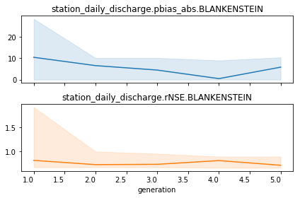
# development of objective functions with generations
_ = run.optimization_populations.plot_generation_objectives()

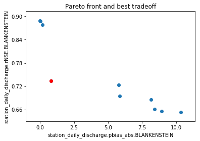
# the Pareto front with the 'best tradeoff' marked
run.optimization_populations.plot_objective_scatter(best=True)
title = plt.title('Pareto front and best tradeoff')

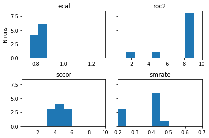
# parameter distribution
_ = run.optimization_populations.plot_parameter_distribution()

Download as Notebook