The forest model 4C - overview
- Principle features
- Light absorption
- Allocation and assimilation
- Water and nutrient balance
- Phenology
- Mortality and regeneration
- Mangement
- Timber grading
- Wood processing model
- Socio-economic analysis
- Species and parameterisation
- References
Principle features
The model 4C (‘FORESEE’ - Forest Ecosystems in a Changing Environment) has been developed to describe long-term forest behaviour under changing environmental conditions (Bugmann et al., 1997). It describes processes on tree and stand level basing on findings from eco-physiological experiments, long term observations and physiological modelling. The model includes descriptions of tree species composition, forest structure, total ecosystem carbon content as well as leaf area index. The model shares a number of features with gap models, which have often been used for the simulation of long-term forest development. Establishment, growth and mortality of tree cohorts are explicitly modelled on a patch on which horizontal homogeneity is assumed.
Important features of the model are:
- the explicit simulation of water and nutrient availability as perceived by individual trees, based on the assumption of scramble competition (Krebs, 1994)
- the transport of heat and water in a multi-layered soil is explicitly calculated, as well as carbon and nitrogen dynamics based on the decomposition and mineralisation of organic matter (Kartschall et al., 1990; Grote and Suckow, 1998).
- The annual course of net photosynthesis is simulated with a mechanistic formulation of net photosynthesis as a function of environmental influences (temperature, water and nitrogen availability, radiation, and CO2) where the physiological capacity (maximal carboxylation rate) is calculated based on optimisation theory (modified after Haxeltine and Prentice, 1996) plus calculation of total tree respiration following the concept of constant annual respiration fraction as proposed by Landsberg and Waring (1997)
- The allocation pattern of annual NPP to the tree organs and tree growth are modelled with a combination of pipe model theory (Shinozaki et al., 1964), the functional balance hypothesis (Davidson, 1969) and several allometric relationships extended to respond dynamically to water and nutrient limitations.
- start and end of the vegetation period are estimated as functions of air temperature and day length (Schaber and Badeck, 2003)
- Establishment and mortality are described based on the concepts proposed by Keane et al. (1996); Loehle and LeBlanc (1996) and Sykes and Prentice (1996). Mortality can be caused either by stress due to negative leaf mass increment in successive stress years or by an intrinsic age-dependent and generic component.
The figure describes the principle interactions of the submodels in 4C.
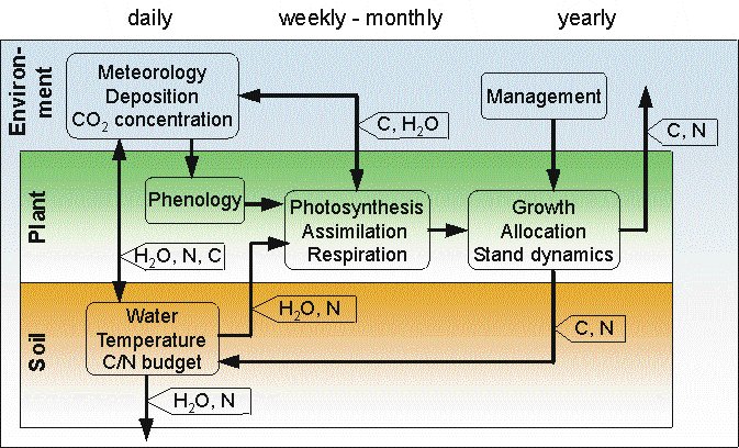
Different integration steps are used for the various submodels, ranging
from a daily time step for soil water dynamics, over one week for soil
carbon and nitrogen dynamics and the simulation of net primary production,
to an annual time step for tree demography and carbon allocation. Hence
the model requires weather data (i.e. temperature, precipitation and solar
radiation) with a daily resolution.
Currently the model is parameterised for the five most abundant tree species of Central Europe (beech, Fagus sylvatica L.; Norway spruce, Picea abies L. Karst., Scots pine, Pinus sylvestris L., oaks, Quercus robur L., and Quercus petraea Liebl., and birch, Betula pendula Roth) and
aspen (Populus tremula (L.), P. tremuloides (Michx.)), Douglas-fir (Pseudotsuga menziesii (Mirb.) Franco), Aleppo pine (Pinus halepensis Mill.), Ponderosa pine (Pinus ponderosa Dougl.).
![]()
Light absorption
The share of any cohort in the total stand’s net photosynthetic assimilation of carbon is proportional to its share of the absorbed photosynthetically active radiation. The total fraction of photosynthetically active radiation absorbed by each cohort is calculated each time stand phenology changes, based on the Lambert-Beer law. There are four different models to calculate light transmission and absorption through the canopy, abbreviated by LM1, LM2, LM3 and LM4 in the following. Whereas LM1 is based on the classical gap model approach that each tree covers the whole patch with its canopy, this simplistic view is refined in LM2 by attributing each cohort/tree a specific projected crown coverage area depending on its dbh. LM2 and LM3 differ in the way the light is transmitted though the canopy and LM4 additionally introduces an average growing season sun inclination angl . Every time phenology changes within the stand, e.g. a species has its bud burst or leaves are colouring, the light transmission through the canopy and accordingly light absorption changes.
![]()
The allocation submodel is based on ideas presented by Mäkelä (1990), with a number of corrections and modifications to make the model sensitive to changing environmental conditions. It is derived for the compartments foliage, sapwood, and fine roots.
The principle of functional balance (Davidson 1969) and the pipe model theory (Shinozaki et al. 1964) together with the principle of mass conservation are used to derive the allocation scheme.
The submodel employs an annual time step.
![]()
Water and nutrient balance
Soil model
The soil is divided into different layers with optional thickness following the horizons of the soil profile. Each layer, the humus layer and the deeper mineral layers, is regarded as homogeneous concerning its physical and chemical parameters. Water content, soil temperature, carbon and nitrogen turnover of each soil layer are estimated as functions of the soil parameters, air temperature, stand precipitation and deposition.
The time step of the soil model is one day due to the great dynamics of the water processes.
Soil water
The soil water content is balanced by a simple percolation model. The input into the first layer is the net precipitation after canopy interception. For each other layer, the input is equal to the percolation water from the above layer. The output is estimated from the percolation water into the next layer, the soil evaporation (up to a certain depth), and the water uptake by roots. If the water content of a layer is greater then the field capacity the percolation water is calculated according to a special water conductivity parameter which is depending on the soil texture (Glugla, 1969;Koitzsch, 1977).
If air temperature is less then 0°C, the precipitation is stored as a water equivalent in a "pool" of snow, which is emptied as a function of temperature. The melt-water will then be added to the uppermost soil layer. In the case of frozen soil no percolation occurs.
Root uptake is limited by the transpiration demand of all trees of the cohort and the plant available water. It is assumed that optimal conditions for water uptake exist only when the water content does not vary by more than 10 percent from the field capacity, otherwise there is a linear reduction of the plant available water (Chen, 1993) . The uptake of each cohort is calculated from its relative share of fine root mass.
Interception
The total interception storage of the canopy is given by a special weighted mean of the species specific interception capacities depending on the leaf area index.This storage is filled by the precipitation and according to the potential evapotranspiration the interception water evaporates (Jansson, 1991). Especially under certain conditions like low temperature and low radiation it is possible, that the interception storage is not emptied during a period of some days. That means, that further precipitation in this period can be intercepted only in a reduced way.
Evapotranspiration
The potential evapotranspiration is calculated on two ways depending on the air temperature: at T ³ 5°C it is calculated by an equation of TURC and at T < 5°C by that of IVANOV (Dyck and Peschke, 1989).
To estimate the potential transpiration of each cohort the potential evapotranspiration is reduced by the interception evaporation. Using the boundary layer parameterization of MONTEITH (Monteith, 1995), the canopy transpiration potential evapotranspiration and the canopy conductance of the forest demand is calculated from the reducedt patch (Haxeltine and Prentice, 1996). The transpiration demand of each cohort is derived by considering its relative conductance.
The drought index of a cohort is defined as the average of the ratios of uptake and demand over the time period of interestd.
Soil temperature
The dynamics of soil temperature are described by a one-dimensional heat conduction equation with spatial and time depending heat capacity and thermal conductivity(Suckow, 1989). The thermal capacity of the soil layer is calculated from the specific heat capacity of the solid soil components, the bulk density and the heat capacity. The thermal conductivity depends on the bulk density and the water content of the soil layer. The upper boundary condition is the surface temperature which is estimated from the air temperature of the last three days. Furthermore, the initialisation of the soil temperature distribution is calculated from the annual temperature wave. The solution of the heat conduction equation with the aid of a non-negative-containing, conservative finite-difference method provides the soil temperature in each soil layer (Suckow, 1986).
Soil carbon and nitrogen
Essential elements in the carbon and nitrogen cycle are the litter and dead fine roots, which supplies the soil with organic matter, their turnover and the nitrogen uptake by plants (King, 1995).
The carbon turnover of the organic matter is the dominant process influenced by water content, soil temperature, and pH value (Franko, 1990; Kartschall, et al., 1990). It provides the energy for the whole turnover of the organic matter and determines the nitrogen turnover. The primary organic matter (needle and foliage litter, twigs , branches, and dead fine roots) decomposes to humus and the mineralization of these organic fractions results in mineral bounded nitrogen and CO 2 which returns to the atmosphere (Goto, et al., 1994). These processes are described as first order reactions (Grote, et al., 1999). Depending on the carbon and nitrogen content of the organic matter and the substrat specific turnover rates, the carbon and nitrogen pools in the soil can be estimated (Running and Gower, 1991).
Furthermore, based on the plant uptake of mineral nitrogen and its transport by water the ammonium and nitrate pools are balanced. This delivers the outflow of nitrogen from the rooted zone.
![]()
The phenolgy model is based on simple interactions between inhibitory and promotory agents that are assumed to control the developmental status of a plant. It is known that temperature and photoperiod play a prominent role. Temperature, for instance, can act through pure physical mechanisms like its influence on viscosity and diffusion. Moreover, synthesis of proteins usually has an activation energy or temperature and an optimal temperature beyond that synthesis rates decrease again ( Vegis 1973, Johnson and Thornley 1985 ). Photoperiod has been observed to be the driving force of a biochemical trigger acting through the phytochrome system (Waring 1956, Nitsch 1957, Perry 1971, Heide 1993a, 1993b ). From these simple but basic principles a model for the abundance or concentration of an inhibitory and a promotory compound can be formulated.
![]()
Mortality and regeneration
The mortality model of 4C considers two kinds of mortality. The so called ‘age related’ mortality basing on life span corresponds to the intrinsic mortality developed by (Botkin, 1993). The response of trees to growth suppression is described by a carbon-based stress mortality.
The regeneration model describes the processes of seed germination, growth and mortality of seedlings, and the recruitment of seedlings into the tree cohorts. Furthermore, the growth and mortality of planted saplings is described with the same model. Growth of each seedling or sapling cohort is updated annually. Net primary production and phenology are simulated similarly to those of older tree cohorts, using radiation, temperature, CO2 concentration, water and nutrient availability as inputs. When the simulated height of the seedlings exceeds an arbitrary threshold value, the entire cohort is then transformed into a regular tree cohort.
![]()
Management
With 4C management of mono- and mixed species forests can be simulated. For this purpose, a number of thinning (thinning from below, thinning from above), harvesting (clear cut, shelterwood) and regeneration strategies (natural regeneration, planting) are implemented (Lasch et al. 2005). Furthermore, short rotation coppice is implemented.
![]()
Timber grading
For provision of information about timber grades of standing and harvested biomass an algorithm is implemented, which delivers a list of all timber products which are available from harvested trees but also standing volume. For this purpose a variety of diameter, height and volume calculations were carried out to assort a stem into different types of wood:
- Stem wood
- Stem segments of various length
- Industrial wood of various length
- Fuel wood
![]()
Wood processing model
The Wood Processing Model (WPM) estimates the carbon content in different timber products and such carbon reservoirs as landfill and atmosphere over the given number of years. As input values WPM uses the pre-estimated amount of harvested wood from the 4C simulation, assumed a forest management was accomplished. A spinup file can be used to initialize single product, landfill and atmosphere pools with realistic values. First, the harvested wood is sorted into different timber grades which then are rearranged into different timber product groups.
Then the product group carbon flow is simulated over the number of simulation years. The product groups have different life spans. The life span functions determine the half-life period of timber and therefore the amount of timber which will be yearly removed from the product groups. The timber removed from the product groups is partly recycled and returns into the timber cycle labelled as timber of age 0. The carbon cycle ends on landfill areas, by burning and hence in the atmosphere. A fixed percentage rate from the landfill carbon volatilises to the atmosphere where it accumulates over the years. The model background of WPM is mainly based on Eggers (2002).
Additional the carbon emission from forest management, the reduction of C emission from fossil fuels through the substitution of fossil fuel by wood in energy production and substitution of materials such as steel, concrete and so by wood (from use category one and two) are calculated.
![]()
Socio-economic analysis
The Socio Economic Analysis (SEA) allows analysing a harvest timber and standing stock due to the aspects of costs, revenues and subsidies in a given time frame.
SEA uses the 4C information about the harvested wood, standing stock and silvicultural operations of a simulated area, sorts the input analog to WPM into different timber grades and computes the costs, assets and subsidies per year. Unlike the WPM it analyses also the standing stock in respect to its financial value. As further input SEA needs an input file with the current prices. This file contains timber prices, silvicultural costs and possible subsidies (Fürstenau e.al. 2007).
![]()
At the time 13 forest species and one type of soil vegetation are parameterised :
Fagus sylvatica
Picea abies
Pinus sylvestris
Quercus robur
Betula pendula
Pinus contorta
Pinus ponderosa
Populus tremula
Pinus halepensis
Pseudotsuga menziesii
Robinia pseudoacacia
Eucalyptus globulus
Eucalyptus grandis
Detailed information about the most abundant tree species of Central Europe (beech, Fagus sylvatica L.; Norway spruce, Picea abies L. Karst., Scots pine, Pinus sylvestris L., oaks, Quercus robur L., and Quercus petraea Liebl., and Douglas-fir, Pseudotsuga menziesii (Mirb.) Franco) and their parameters are given in a table.
![]()
References
Botkin, D. (1993). Forest Dynamics: An Ecological Model. Oxford & New York, Oxford University Press.
Bugmann, H., Grote, R., Lasch, P., Lindner, M. and Suckow, F. (1997). A new forest gap model to study the effects of environmental change on forest structure and functioning. Impacts of Global Change of Tree Physiology and Forest Ecosystem. Proceedings of the International Conference on Impacts of Global Change on Tree Physiology and Forest Ecosystems, held 26-29 November 1996, Wageningen. Mohren, G. M. J., et al. Dordrecht, Kluwer Academic Publisher. 255-261.
Chen, C. W. (1993). The response of plants to interacting stresses: PGSM Version 1.3 Model Documentation. Palo Alto, USA, Electric Power Res. Inst.
Davidson, R. L. (1969). Effect of root/leaf temperature differentials on root/shoot ratios in some pasture grasses and clover. Ann. Bot. 33: 561-569.
Dyck, S. and Peschke, G. (1989). Grundlagen der Hydrologie. Berlin, Verlag für Bauwesen.
Eggers, T. (2002). The impacts of manufacturing and utilization of wood products on the European carbon budget. Joensuu, European Forest Institute: 90.
Franko, U. (1990). C- und N-Dynamik beim Umsatz organischer Substanz im Boden. Berlin, Akademie der Landwirtschaftswissenschaften der DDR.
Fürstenau, C., F. Badeck, P. Lasch, M. Lexer, M. Lindner, P. Mohr and F. Suckow (2007). "Multiple-use forest management in consideration of climate change and the interests of stakeholder groups." European Journal of Forest Research 126(2): 225-239.
Glugla, G. (1969). Berechnungsverfahren zur Ermittlung des aktuellen Wassergehaltes und Gravitationswasserabflusses im Boden. Albrecht-Thaer-Archiv 13: 371-376.
Goto, N., Sakoda, A. and Suzuki, M. (1994). Modelling of soil carbon dynamics as a part of carbon cycle interrestrial acosystems. Ecol. Modell. 74: 183-204.
Grote, R., Suckow, F. and Bellmann, K. (1999). Modelling of carbon-, nitrogen-, and water balances in pine stands under changing air pollution and deposition. Changes of Atmospheric Chemistry and Effects on Forest Ecosystems. A Roof Experiment Without Roof. Hüttl, R. F. and Bellmann, K. Dordrecht, Kluwer. 3: 251-281.
Haxeltine, A. and Prentice, I. C. (1996). A general model for the light-use efficiency of primary production. Functional Ecology 10(5): 551-561.
Jansson, P.-E. (1991). Simulation model for soil water and heat conditions. Description of the SOIL model. Uppsala, Swedish University of Agricultural Sciences, Department of Soil Sciences, Division of Agricultural Hydrotechnics.
Johnson, I. R. and J. H. M. Thornley (1985). Temperature dependance of plant and crop processes. Annals of Botany 55: 7-24.
Kartschall, T., Döring, P. and Suckow, F. (1990). Simulation of Nitrogen, Water and Temperature Dynamics in Soil. Syst. Anal. Model. Simul. 7(6): 33-40.
Keane, R. E., Morgan, P. and Running, S. W. (1996). FIRE-BGC - A mechanistic ecological process model for simulating fire succession on coniferous forest landscapes of the northern Rocky Mountains. Ogden, UT, United States Department of Agriculture, Forest Service, Intermountain Research Station.
King, D. A. (1995). Equilibrium analysis of a decomposition and yield model applied to Pinus radiata plantations on sites of contrasting fertility. Ecol. Modell. 83: 349-358.
Koitzsch, R. (1977). Schätzung der Bodenfeuchte aus meteorologischen Daten, Boden- und Pflanzenparametern mit einem Mehrschichtmodell. Z. f. Meteor. 27(5): 302-306.
Krebs, C. J. (1994). Ecology - The experimental analysis of distribution and abundance. New York, Harper & Row.
Landsberg, J. J. and Waring, R. H. (1997). A Generalised Model of Forest Productivity Using Simplified Concepts of Radiation-Use Efficiency, Carbon Balance and Partitioning. Forest Ecology & Management 95(3): 209-228.
Lasch, P., F. W. Badeck, F. Suckow, M. Lindner and P. Mohr (2005). Model-based analysis of management alternatives at stand and regional level in Brandenburg (Germany). Forest Ecology And Management 207(1-2): 59-74.
Loehle, C. and LeBlanc, D. (1996). Model-based assessments of climate change effects on forests: a critical review. Ecological Modelling 90: 1-31.
Mäkelä, A. (1990). Modeling structural-functional relationships in whole-tree growth: resource allocation. Process modeling of forest growth responses to environmental stress. R. K. Dixon, R. S. Meldahl, G. A. Ruark and W. G. Warren. Portland, Oregon, Timber Press: 81-95.
Monteith, J. L. (1995). Accomodation between transpiring vegetation and the convective boundary layer. Journal of Hydrology 166: 251-263.
Running, S. W. and Gower, S. T. (1991). FOREST-BGC, A general model of forest ecosystem processes for regional applications II. Dynamic carbon allocation and nitrogen budgets. Tree Physiology 9: 147-160.
Schaber, J. and Badeck, F.-W. (2003). Physiology based phenology models for forest tree species in Germany. Intern. J. Biometeorol. 47(4): 193-201
Shinozaki, K., Yoda, K., Hozumi, K. and Kira, T. (1964). A quantitative analysis of plant form - the pipe model theory. I. Basic analysis. Jap. J. of Ecology 14: 97-105.
Suckow, F. (1989). Ein Modell zur Berechnung der Bodentemperatur im Rahmen des Basismodells Boden (BAMO). Tag.-Ber., Berlin, Akad. Landwirtsch.-Wiss. DDR.
Suckow, F. (1986). Ein Modell zur Berechnung der Bodentemperatur unter Brache und unter Pflanzenbestand. Berlin, Akademie der Landwirtschaftswissenschaften der DDR.
Sykes, M. T. and Prentice, I. C. (1996). Carbon storage and climate change in Swedish forests: a comparison of static and dynamic modelling approaches. Forest ecosystems, forest management and the global carbon cycle. Apps, M. and Price, D. T. Berlin Heidelberg New York, Springer. 40: 69-78.
![]()
about 4C | news | 4C guide | theory | applications | publications | contact