The base for visualisation of results of the numerical experiments is the plane
![]() , each point of which can be considered as a
climatic scenario (see Figs. 5, 6 and 8). For
instance, the point
(
, each point of which can be considered as a
climatic scenario (see Figs. 5, 6 and 8). For
instance, the point
(![]() ) means
that the mean temperature of the vegetation period and its variance increase by
) means
that the mean temperature of the vegetation period and its variance increase by
![]() C and
C and ![]() C respectively (in comparison with their
contemporary values). Using the crop production model and the statistical
weather generator (the mean temperature and its variance are the parameters of
generated stochastic process) 300 Monte-Carlo experiments were carried out for
each point of the plane. In fact, using these experiments we construct an
empirical distribution for the crop yield y. Then the distribution is tested
as a normal one and the sample mean of the crop production
C respectively (in comparison with their
contemporary values). Using the crop production model and the statistical
weather generator (the mean temperature and its variance are the parameters of
generated stochastic process) 300 Monte-Carlo experiments were carried out for
each point of the plane. In fact, using these experiments we construct an
empirical distribution for the crop yield y. Then the distribution is tested
as a normal one and the sample mean of the crop production ![]() and its
sample variance s are calculated. The procedure is repeated again for the
next
and its
sample variance s are calculated. The procedure is repeated again for the
next ![]() and
and ![]() . As a result, we obtain the functions
. As a result, we obtain the functions
![]() and
and ![]() ,
the isolines of them are depicted in the plane
,
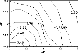
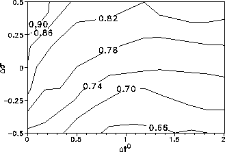
the isolines of them are depicted in the plane ![]() in Figs. 5 and 6. The origin of co-ordinates in this plane
corresponds to the contemporary climate. Since the crop yield unit is t/ha,
in Figs. 5 and 6. The origin of co-ordinates in this plane
corresponds to the contemporary climate. Since the crop yield unit is t/ha,
![]() and s are measured with the same unit. Note that the increase of
number of the experiments does not really change these pictures.
and s are measured with the same unit. Note that the increase of
number of the experiments does not really change these pictures.

Figure 5: Isolines of the mean crop production (in tons per hectare).

Figure 6: Isolines of the crop production variance (in tons per hectare).
In fact, we use the crop model like some non-linear filter which transforms a set of stochastic climatic time-series into a set of crop yield values. Since suitable probabilistic measures have been defined on both sets, the filter maps one onto the other, and using Monte-Carlo experiments we define the functional connection between the moments of corresponding probabilistic distributions:
As mentioned above, if the state of agriculture system is determined by the
scalar value of the crop yield y, then the event ![]() is considered as an ``agricultural disaster''. The critical value
is considered as an ``agricultural disaster''. The critical value ![]() is
determined by economic and social arguments laying outside of the considered
problem. For instance,
is
determined by economic and social arguments laying outside of the considered
problem. For instance, ![]() t/ha for Kursk region. This
choice has been made from the social and historical arguments (rural population
in the Central Russia was perceiving a crop yield less than 1.5 tons per
hectare as a disaster). The homeostatic domain and its boundary are defined in
this case as
t/ha for Kursk region. This
choice has been made from the social and historical arguments (rural population
in the Central Russia was perceiving a crop yield less than 1.5 tons per
hectare as a disaster). The homeostatic domain and its boundary are defined in
this case as ![]() .
.
Keeping in mind the risk definition we can formulate the following
probabilistic statement: let ![]() be the probability of
the event
be the probability of
the event ![]() . Then
. Then ![]() ,
where
,
where ![]() is the
corresponding percentile of the probability distribution Pr with the
arithmetic mean
is the
corresponding percentile of the probability distribution Pr with the
arithmetic mean ![]() and the variance
and the variance ![]() . The
corresponding statistical test has shown that this distribution is very close
to the normal one. If the line
. The
corresponding statistical test has shown that this distribution is very close
to the normal one. If the line
![]() is drawn in the plane
is drawn in the plane
![]() (Fig. 7) then it divides the plane
on two domains corresponding to normal and catastrophic states.
(Fig. 7) then it divides the plane
on two domains corresponding to normal and catastrophic states.

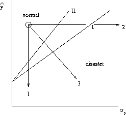
Figure 7: Normal and catastrophic (disaster) domains. Line I:
![]() , line II:
, line II: ![]() ,
, ![]() .
.
Let us assume that under some climate change only the mean crop yield was
changed (the trajectory ![]() in Fig. 7), and, as a result,
that the system was found in the catastrophic domain. On the other hand, the
same result obtains if the mean crop yield is not changed, but only the
variance increases (the trajectory
in Fig. 7), and, as a result,
that the system was found in the catastrophic domain. On the other hand, the
same result obtains if the mean crop yield is not changed, but only the
variance increases (the trajectory ![]() ). In many agricultural
forecasts only the first case is considered for the same reason, and the second
case is forgotten, which is also possible. In actuality both the mean crop
yield and its variance are changed (the trajectory
). In many agricultural
forecasts only the first case is considered for the same reason, and the second
case is forgotten, which is also possible. In actuality both the mean crop
yield and its variance are changed (the trajectory ![]() ). At last,
since the increase of the percentile a corresponds to the decrease of risk
level, then the catastrophic domain must also increase (line II in
Fig. 7).
). At last,
since the increase of the percentile a corresponds to the decrease of risk
level, then the catastrophic domain must also increase (line II in
Fig. 7).
By setting ![]() and
and ![]() using the dependencies
using the dependencies
![]() and
and ![]() , we
have
, we
have ![]() . The functions f and
. The functions f and ![]() are known (see Figs. 5 and 6), therefore
are known (see Figs. 5 and 6), therefore
![]() can be calculated. The results are shown in Fig. 8, where the isolines of R
are drawn in the plane
can be calculated. The results are shown in Fig. 8, where the isolines of R
are drawn in the plane ![]() .
.
Figure 8: Isolines of the annual risk(in %).
We can see that, for instance, the annual 3%-risk level remains practically
constant when the temperature rises by ![]() C (if the variance
is not changed). But the risk rises very fast if the variance increases also
(even if the change of mean temperature would be very small)! This is one
more argument confirming that a forecast of temperature variance is a very
important problem.
C (if the variance
is not changed). But the risk rises very fast if the variance increases also
(even if the change of mean temperature would be very small)! This is one
more argument confirming that a forecast of temperature variance is a very
important problem.
Generally speaking, the information contained in Fig. 8 is sufficient to predict the change of admissible risk for any climatic scenario. We can see that the most dangerous situation would be when both the mean temperature and its variance would be increased in a similar way. In this case the probability of disaster increases very fast. But what is the probability that this case could be realised?
Let us come back to the climate models. Today we cannot decide, what kind of
model gives the best predictions of the future climate. This is, in particular,
true for the prediction of statistical characteristics. Of course, we could
combine these models to construct some sort of ``optimal predictor'', but what
kind of criterion do we have to use? We cannot be sure that an average
prediction would be the optimal one. A possible approach is to indicate some
intervals for probable change of climatic parameters and to suppose that all
the changes are equiprobable (``microcanonical ensemble''). This implies that
in our case study the ![]() -set in the plane
-set in the plane
![]() is a simple rectangular domain
is a simple rectangular domain
![]() (Fig. 8, and the distribution
(Fig. 8, and the distribution ![]() is a simple rectangular
distribution. In order to calculate the annual risk under climate change the
function
is a simple rectangular
distribution. In order to calculate the annual risk under climate change the
function ![]() must be integrated over the
predicted domain of possible climate change, A, so that
must be integrated over the
predicted domain of possible climate change, A, so that
![]()
where ![]() is an area of the domain S,
is an area of the domain S, ![]() . Here the annual risk
. Here the annual risk
![]() turns out to be 7%.
turns out to be 7%.
Since the ``risk'' probability is the result of the convolution of many factors and processes, and of only two moments of the real distribution, we can formulate a plausible hypothesis: the final result (risk assessment) depends very weakly on the form of such a distribution.
Finally, we can say that there are a lot of other works (see, for instance, [12]-[16]) dealing with the problem of estimating the impact of climate change on agro-ecosystems. Their authors are usually using different climatic scenarios and different methods of forecasting. It is no wonder that there is a large inconsistency in their quantitative forecasts (even if they use similar scenarios). On the other hand, there is one common qualitative item among them: they all forecast that the climate change would cause a significant drop of the potential productivity of basic crops (especially, spring ones) in many agricultural regions of the World. Note that, as a rule, only the change of mean climatic parameters are taken into account in the forecasts.