Based on the analytical analysis, the system is analysed numerically in
respect to the positions and number of stable equilibria. Phase portraits showing trajectories in the ![]() -domain
give a visual impression of the system behaviour. The equilibria of the system are easily obtained by plotting the two functions
I:
-domain
give a visual impression of the system behaviour. The equilibria of the system are easily obtained by plotting the two functions
I:![]() (eq. (11)) and II:
(eq. (11)) and II:![]() (eq. (35)) and determining their intersection points in the phase space. The maximum number of possible equilibria is
restricted to five, because both functions I and II are unimodular ones and
therefore intersect at a maximum of four points in
(eq. (35)) and determining their intersection points in the phase space. The maximum number of possible equilibria is
restricted to five, because both functions I and II are unimodular ones and
therefore intersect at a maximum of four points in ![]() . Together with the ``naked'' equilibrium one gets five as an upper boundary for the number of stationary
solutions.
. Together with the ``naked'' equilibrium one gets five as an upper boundary for the number of stationary
solutions.
For a certain set of
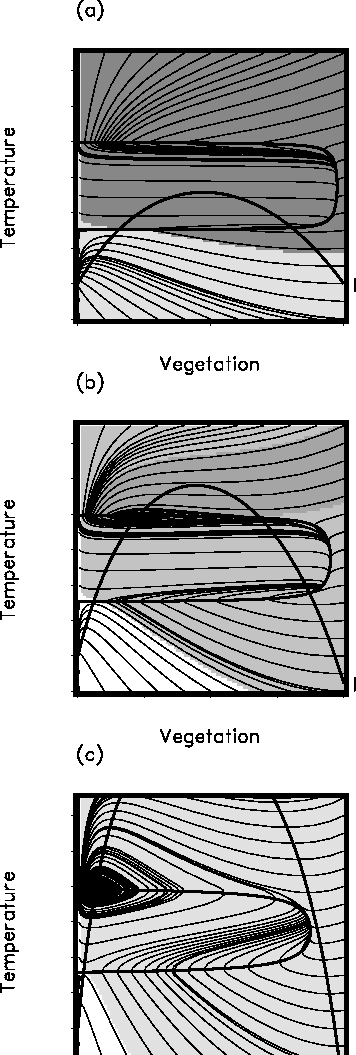
parameters we have a phase portrait as in Fig. 11a: two of the three possible
equilibria are stable, the ``cold desert'' with N=0 and the ``cold'' planet with N>0. The
unstable equilibrium separates the two basins of attraction. If A is increased, but ![]() is fixed,
the phase portrait changes according to Fig. 11b, where three stable equilibria
exist (``cold desert'' ``cold '' planet, and ``hot'' planet). A further increase of A reduces their number to two (Fig. 11c).
is fixed,
the phase portrait changes according to Fig. 11b, where three stable equilibria
exist (``cold desert'' ``cold '' planet, and ``hot'' planet). A further increase of A reduces their number to two (Fig. 11c).

Figure 11: Phase portraits for increasing A and fixed ![]() . (a): ``cold desert'' and ``cold'' planet are stable equilibria, (b) ``cold desert'' ``cold'' and ``hot'' planet are stable, (c) ``cold desert'' and ``hot'' planet are stable. Curve I:
. (a): ``cold desert'' and ``cold'' planet are stable equilibria, (b) ``cold desert'' ``cold'' and ``hot'' planet are stable, (c) ``cold desert'' and ``hot'' planet are stable. Curve I: ![]() , and II:
, and II: ![]() . The different shaded areas denote the basins
of attraction.
. The different shaded areas denote the basins
of attraction.
Since we would like our planet to be similar to the Earth, we shall use real values for estimation of the model parameters.
It is known for Earth that ![]() ,
, ![]() for land and
for land and
![]() for ocean. Since our planet has no ocean,
without loss of generality, we can put
for ocean. Since our planet has no ocean,
without loss of generality, we can put ![]() . The time step
of the model is equal to 1 year
. The time step
of the model is equal to 1 year![]() sec, then
sec, then ![]() in
the corresponding units. The albedo for ``naked'' Earth (white sands) is
in
the corresponding units. The albedo for ``naked'' Earth (white sands) is
![]() , and for ``green'' Earth
, and for ``green'' Earth ![]() [2].
[2].
About the role of atmospheric carbon: the ``greenhouse'' effect. In agreement with Petoukhov[8],
![]() and
and ![]() or
or ![]() , so that
, so that
![]()
if C is measured in Gt. Note that ![]() .
.
The temperature of the ``cold desert'' for Earth is determined by
![]()
Here ![]() . On the other hand, the contemporary temperature
is
. On the other hand, the contemporary temperature
is ![]() . Note that in this case the mean albedo
. Note that in this case the mean albedo ![]() , so
that
, so
that ![]() , and the equilibrium temperature for a planet without atmosphere
would be
, and the equilibrium temperature for a planet without atmosphere
would be
![]()
Containing ![]() and
and ![]() , the atmosphere increases the
temperature (the ``greenhouse effect'' This increase can be obtained as a result of
the reduction of the coefficient
, the atmosphere increases the
temperature (the ``greenhouse effect'' This increase can be obtained as a result of
the reduction of the coefficient ![]() ; when we introduce some ``effective''
; when we introduce some ``effective''
![]() denoted as
denoted as ![]() :
:
![]()
where ![]() is a decreasing function, taking into account the role
of
is a decreasing function, taking into account the role
of ![]() ,
, ![]() is the similar function for water vapour with
concentration W. Obviously,
is the similar function for water vapour with
concentration W. Obviously, ![]() . For
C=610Gt the corresponding value is
. For
C=610Gt the corresponding value is ![]() .
.
If we neglect the water vapour contribution, then
![]() ,
just as the real temperature is
,
just as the real temperature is ![]() . It shows that this
contribution is very important, and we must include
it in our consideration (in some implicit changing
. It shows that this
contribution is very important, and we must include
it in our consideration (in some implicit changing ![]() ). From this
condition
). From this
condition
![]()
we get ![]() , and
, and ![]() . But
only considering
. But
only considering ![]() in the atmosphere, then
in the atmosphere, then
![]()
and
![]()
Since
![]()
where ![]() , then
, then
![]()
We assume that the contemporary state of the biosphere is an equilibrium. We consider the current productivity of the biosphere as the equilibrium one. Here and hereafter we use the data from [12].
The ``soil'' compartment was omitted in our model. Its influence can be
described by an increase of the residence time of carbon in the biota. On the
other hand, the relatively large part of dead organic matter (![]() )
is returned very rapidly to the atmosphere. For this reason, as an initial
approximation, we can forget about the ``soil'' compartment and consider the
following estimations:
)
is returned very rapidly to the atmosphere. For this reason, as an initial
approximation, we can forget about the ``soil'' compartment and consider the
following estimations:

so that the residence time of carbon in the biota is equal to 12.5 years.
The tolerance interval for photosynthesis is ![]() , and
, and
![]() (for a parabolic approximation of the growth function).
Since
(for a parabolic approximation of the growth function).
Since ![]() , then
, then
![]()
And from
![]()
we get
![]() .
And, finally, from
.
And, finally, from
![]()
we get ![]() Gt.
Gt.
| parameter | value | units |
| S | 340 | |
| k | | |
|
| | |
|
| 0.4 | |
|
| 0.1 | |
|
| 0.6 | |
|
| 750 | Gt |
|
| 600 | Gt |
|
| 5 | |
|
| 40 | |
| A | 1360 | Gt |
| m | 0.08 | 1/year |
|
| 80 | Gt/year |
We have for our planet: ![]() , i.e. the total amount
of carbon is less than three times compared to its critical value and equilibria
with
, i.e. the total amount
of carbon is less than three times compared to its critical value and equilibria
with ![]() can exist.
Remembering the formula for
can exist.
Remembering the formula for ![]() , we can test the value
, we can test the value ![]() . It is
equal to
. It is
equal to ![]() (for
(for ![]() Gt). And finally we must note that all
values N, C, etc. are measured in Gt (
Gt). And finally we must note that all
values N, C, etc. are measured in Gt (![]() tons).
tons).
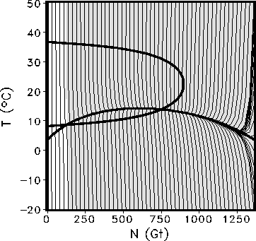
Fig. 12 plots the
phase portrait corresponding to the parameter setting for Earth
summarized in Tab. 1. The phase portrait is similar to Fig. 11a, where two equilibria
(the cold desert and the cold planet with vegetation) are stable for the
given A. But note that for the present state of the Earth the planet without vegetation ![]() for any T is stable preventing life arising from the ``dead'' planet state. Leaving the basin of attraction of
for any T is stable preventing life arising from the ``dead'' planet state. Leaving the basin of attraction of ![]() by, e.g., perturbation of N to a value
below a critical threshold leads to a complete extinction of vegetation on Earth.
by, e.g., perturbation of N to a value
below a critical threshold leads to a complete extinction of vegetation on Earth.

Figure 12: Phase portrait for the system with parameter settings according
to real Earth scenario.